Seismically Guided Fracture Characterization

Introduction

In the future, there will be greater dependency on producing oil and gas from fractured reservoirs. Characterization and forecasting in fractured reservoirs are two of the most challenging topics in the oil and gas industry. Managing such reservoirs requires construction of representative reservoir models that can handle both fracture and matrix systems and their interaction correctly. Data integration fro m multiple disciplines is required for construction of these reservoir models.

The flow behavior in reservoirs may be dominated (positively or negatively) by the existence of fractures on the order of millimeters in thickness that are directly observed only at the wells utilizing some types of image logs or core photos. Fracture drive can be further implied through well testing when a high permeability interpretation of a well test is not directly supported by any other log measurements. Further, to properly model the fluid flow in fractured reservoirs, one must model both the flow due to the primary matrix rock that may be on the order of 1-m by 50-m by 50-m matrix blocks and the effect due to the small-scale fractures that may consist of oriented sets of fractures on the size order of millimeters.

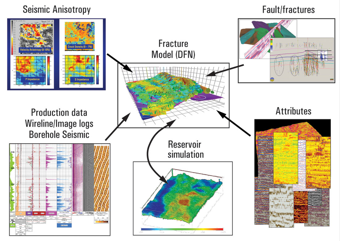
A summary of how surface seismic data can be integrated into building a fracture model is shown in Figure 1. Surface seismic data can impact fracture scale all the way from km-type measurements (faults) through scales approaching a seismic wavelength of ten to hundreds of meters (fractures + attributes), and finally to subseismic scales (seismic azimuthal anisotropy). Of course, the key to fracture modeling is to be able to integrate the various measurements at all scales and produce flow simulations that match the production history of the field.

Fault and Fracture Mapping

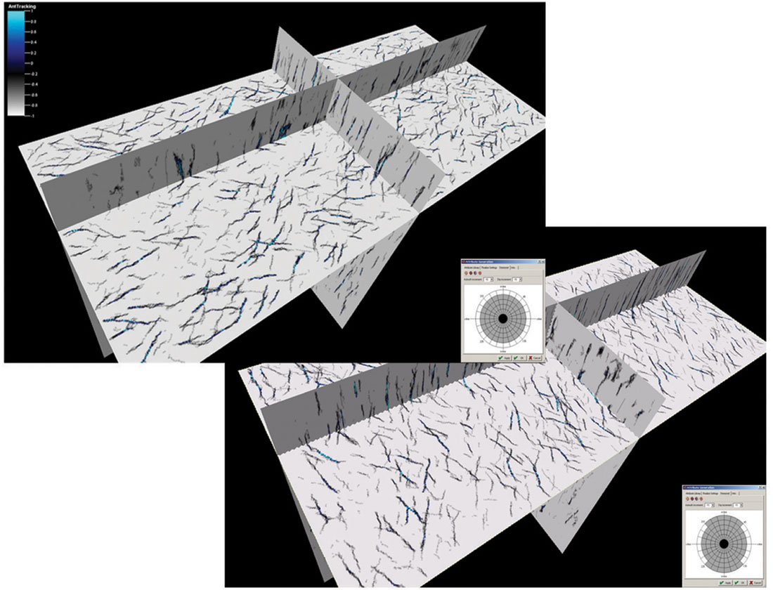
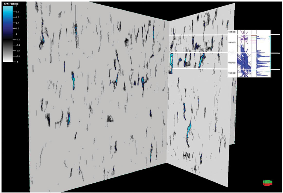
Fault systems that contribute to the structural setting of a field are generally interpreted manually. Discontinuity evaluation software that relies on pattern recognition techniques has recently become available that can help automate fault interpretation (km scale) and, in addition, attempt to map features that are on a scale approaching a seismic wavelength (30-100 m). One such technique, implemented in the Petrel geological modeling software package, is called ant tracking. The results of using ant tracking in a workflow that involves training the ant – tracking parameters using image and core data are shown in Figures 2 and 3. Figure 2 show that mapping subvertical dipping features using all strike azimuths in the ant – tracking results in mapping a dominant N-S fault system. Restricting the azimuth range to E-W in the ant tracking reveals a fracture system trending NE-SW. A vertical section through the ant density cube is shown in Figure 3, and the correlation between the fracture intensity interpreted from a Formation MicroImager (FMI) log and the ant density at a well location is apparent.

Attributes

Seismic attribute processing can illuminate features within the original seismic data that correlate with faulting and fracture corridors. These processing methods can discriminate amplitude and frequency variation by signal analysis on individual seismic traces; for example, a fracture corridor could cause local attenuation of high frequencies as measured above and below the zone. Multitrace attributes extend the analysis to include local orientation and signal similarity estimates. Earlier investigators showed that dip magnitude and dip azimuth could illuminate subtle faults that have a displacement significantly less than the size of a seismic wavelet. Edge detection methods measure lateral changes in seismic waveforms and amplitude. More recently, curvature attributes have been found to be useful in delineating faults and predicting fracture orientation and distribution.

No one “magic bullet” attribute has been shown to always indicate natural fractures, though some are promising under certain geologic conditions. Current research indicates that combinations of various attributes can be used with better success, particularly in “hard rock” environments. This success rate can be increased with the inclusion of additional fracture data, such as FMI or reservoir engineering data, to help constrain the interpretation of these attributes. This makes the development of discrete fracture network (DFN) models extremely important when identifying fracture trends and swarms.

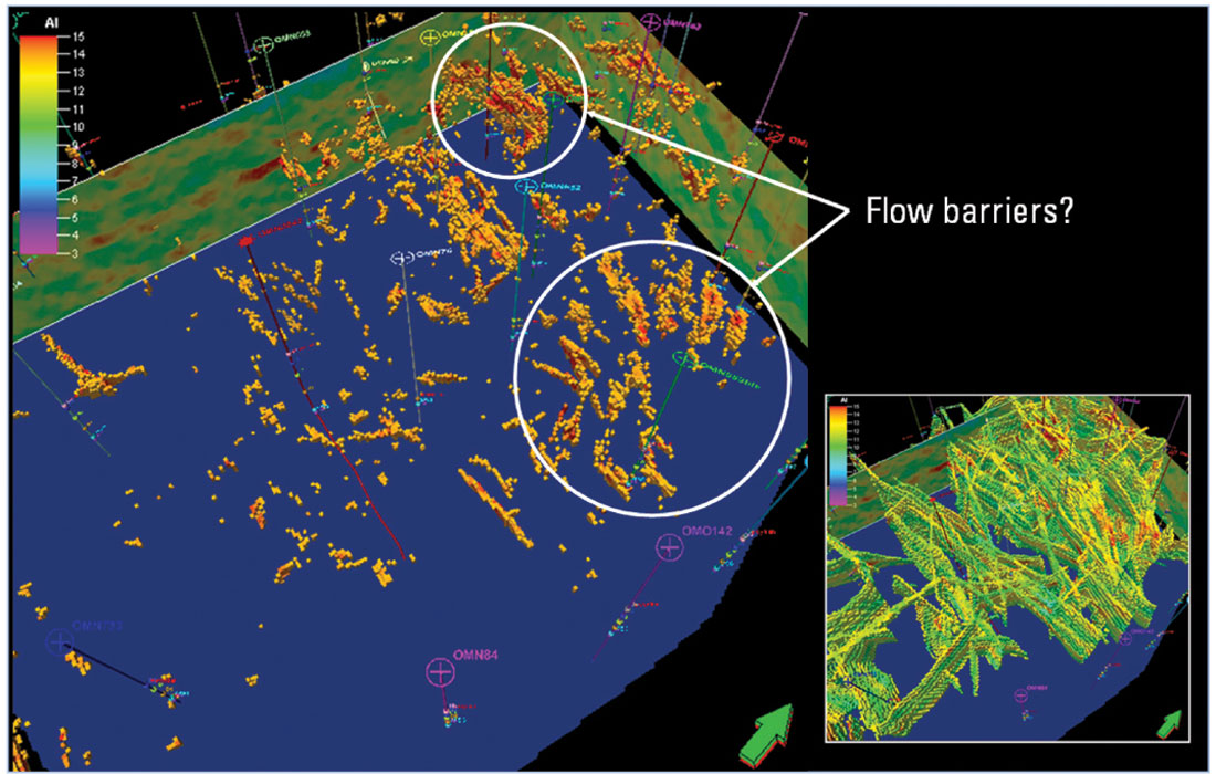
Figure 4 shows how a seismic impedance attribute can be used to infer which faults (picked using the ant-tracking technique mentioned above) are sealing and, therefore, represent flow barriers or equivalently low permeability zones. In this figure, a threshold was applied to the impedance cube to allow only high impedance in the vicinity of the faults. A distance-to-fault attribute is shown in the lower right corner. Conversely, a low impedance threshold could indicate zones of high permeability, indicating flow conduits.

Seismic Anisotropy

When the fractures are much smaller than the seismic wavelength, we can not image them directly. Rather, the presence of small-scale fractures is inferred from observed seismic anisotropy using effective media theories. See Lynn (2004) for additional discussion. In general, a rock physics model is used that relates porosity, crack density, and additional rock parameters to seismic anisotropy. Among the more popular models are Hudson’s penny- shaped cracks model (1981) and Schoenberg and Sayers (1995) access compliance model. New developments in well log data acquisition enable the calibration of such rock models to azimuthal sonic and shear log data, as well as FMI images. See, for example, Priuol et al. (2007). The observed seismic anisotropy is used to infer the amount of cracks and their orientation with respect to the rock model. It is important to note that azimuthal anisotropy can also be caused by triaxial stress state in the sediment, and thus interpretation of such observation should be done with respect to the state of stress in the basin.

In general, when referring to seismic anisotropy for fracture detection, both P-wave and S-wave information can be used to infer the presence of aligned vertical fractures having a subseismic scale.

From P-wave seismic data, the azimuthal anisotropy is derived from azimuthal variations of traveltimes (kinematics) and amplitude (dynamic). When analyzing traveltime data, we look for a 90° variation between fast-to-slow on offsets approximately equal to target depth that arise from aligned ordered heterogeneities that are very small relative to the wavelength. The analysis of amplitude vs. angle and offset (AVAZ) is used to derive relative contrasts in anisotropic parameters along a layer interface. It is important to note that the AVAZ method often provides high-resolution estimates of anisotropy (between the seismic bandwidth of the wavelet). The traveltime method will provide lower resolution. Note also that kinematic and dynamic information can be integrated in a consistent manner as discussed by Bachrach et al. (2006). We see that little or no change of phase over azimuth and little or no change of frequency with azimuth (fixed offset) is observed.

The second type of seismic anisotropy is based on the observation that shear waves split into two shear waves upon encountering these fractures. In the presence of unequal horizontal stresses and/or aligned vertical fractures, an arbitrarily polarized vertically propagating shear wave will split into the fast shear wave, polarized parallel to the stiff direction of the rock, and the slow shear wave, polarized perpendicular to the fast shear wave. The polarization (particle motion direction) of these split shear waves documents the stiff direction of the rock and the compliant direction of the rock. In addition, AVAZ analysis of shear-wave data (and PS data) can also be preformed performed if data quality is sufficient. It is also important to note that as shear waves are not sensitive to fluids, in many cases, case seismic anisotropy inferred from shearwave data can be correlated to crack density distribution without the additional complexity of analyzing pore and crack fluid effects on anisotropy.

Azimuthal variations in PP seismic signatures can be ambiguous as to whether heterogeneity (different rocks along the different raypaths) or anisotropy is causing the signature. Therefore, many people prefer to look at split shear waves, for they have traveled (reasonably) the same path and any difference in their amplitude, traveltime, phase, or frequency is due to the anisotropy.

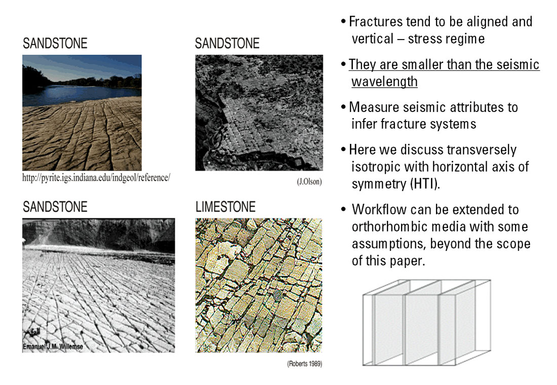
Figure 5 shows four different outcrops exhibiting aligned vertical fractures both in sandstone and carbonate reservoirs, and Figure 6 shows the results of inferring fracture density and orientation from azimuthal variations in velocity from PP-wave data and shear-wave birefringence from PS-wave data. Note that reconciling the different interpretations produced from these seismic measurements and deciding what impact they will have on conditioning the discrete fracture network (DFN) requires integration with the well, production, and image data.

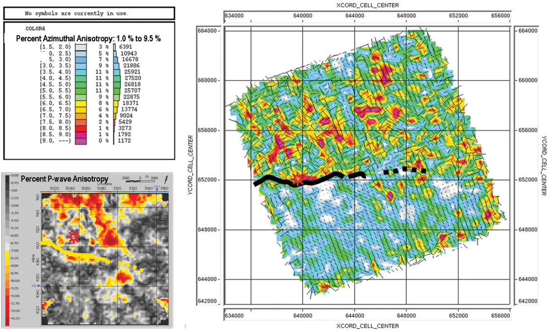
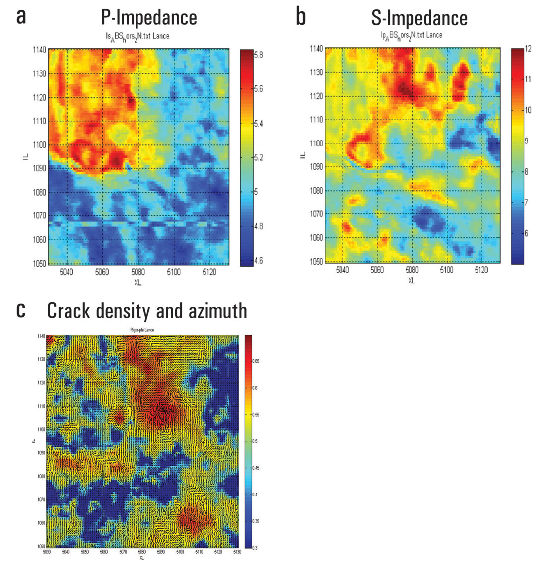
Figure 7 present images of P-impedance, S-impedance, and crack density estimated using rock physics models and AVAZ analysis (After Sengupta and Bachrach, 2006). In this case, orientation is derived from AVAZ analysis.

Discrete Fracture Modeling

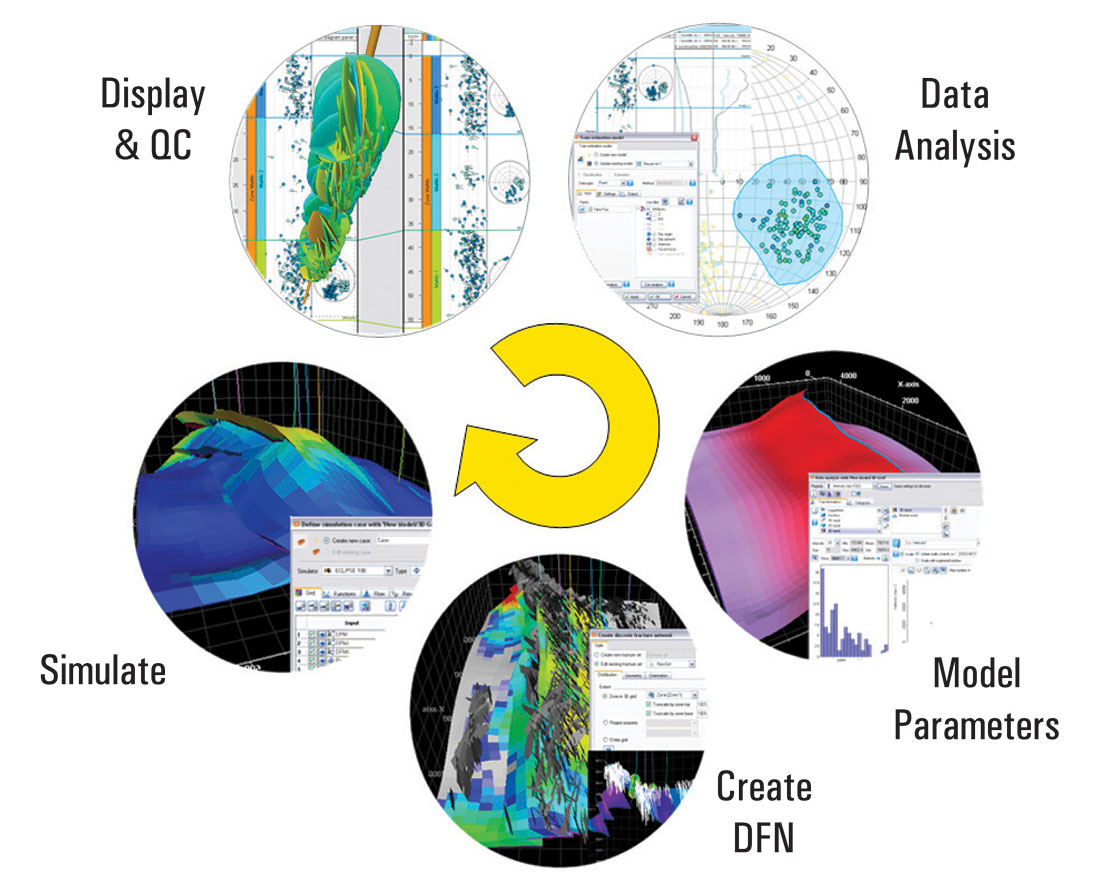
There are six key workflow elements that must be addressed when building a discrete fracture model that can be used to simulate fluid flow and help in production history matching.

1. Deriving, analyzing, and understanding the “fracture signature” from various data inputs and interpretations. These include well image logs, seismic attributes, well tests, cores, and various others.
2. Building the 3D geologic model (structure and facies) and analyzing the data that will be used to statically model the 3D fracture patterns.
3. Characterizing the 3D fracture set networks.
4. Upscaling the model, creating the dual porosity and permeability inputs to the reservoir simulator and then simulating.
5. Validating the simulation model though well tests and production history match.
6. Iterating through the workflow to keep the model up to date.

These have been implemented in the discrete fracture network capability in the Petrel package illustrated in Figure 8.

Summary

Efficient fracture modeling requires both deterministic and stochastic elements to be integrated into a model so that multiple flow simulations can be run and matched to production history. Seismic data can provide input on both the deterministic (fracture corridors and fault systems) and the stochastic elements (stress field using seismic anisotropy).

Acknowledgements

We want to thank all our colleagues in WesternGeco and Schlumberger who have contributed to the development of the work flow. In particular, Mahmood Akbar, Donatella Astratti, Colin Daly, Paul Ras and Lars Sonneland have developed and tested a number of the technologies discussed in the paper.