Overview
“We have so much dynamic range now that …” – and then you fill in the blanks. This is perhaps one of the most frequently mis-used phrases in our industry today. This prelude has been used to justify many excuses for poor acquisition practices from the grouping of analog geophones to the use of abnormally large charges.
In fact, our instruments for field acquisition have evolved considerably over the past twenty years. But the true value of the gains we have made is poorly understood amongst the geophysical industry. In this article, we attempt to highlite the differences between current technology and older technology . We will demonstrate that, although new instruments offer many advantages, we would be foolish to ignore the limits of dynamic range in our seismic system.
We will compile a list of common statements (some fact, some myth) regarding instrumentation, and will endeavour to separate those which are true in today’s world of acquisition.
IFP Instruments – from whence did we evolve?
First let us see where we started in the early 1980’s. One of the leading instruments at the time was the DFS V. Figure 1 is a simple block model showing the basic components of this system. In this system, electronic signals were generated by groups of geophones distributed in the field and these signals were propogated through long analog cables to a central recording truck that housed all of the electronics to manipulate, measure and record these signals. While the signal travelled down these cables, it was vulnerable to induction noise and transmission losses and distortions. Also the cables were one of the greatest sources of “crossfeed” – a weak, induced copy of signal from one pair of wires into the signal on an adjacent pair of wires.
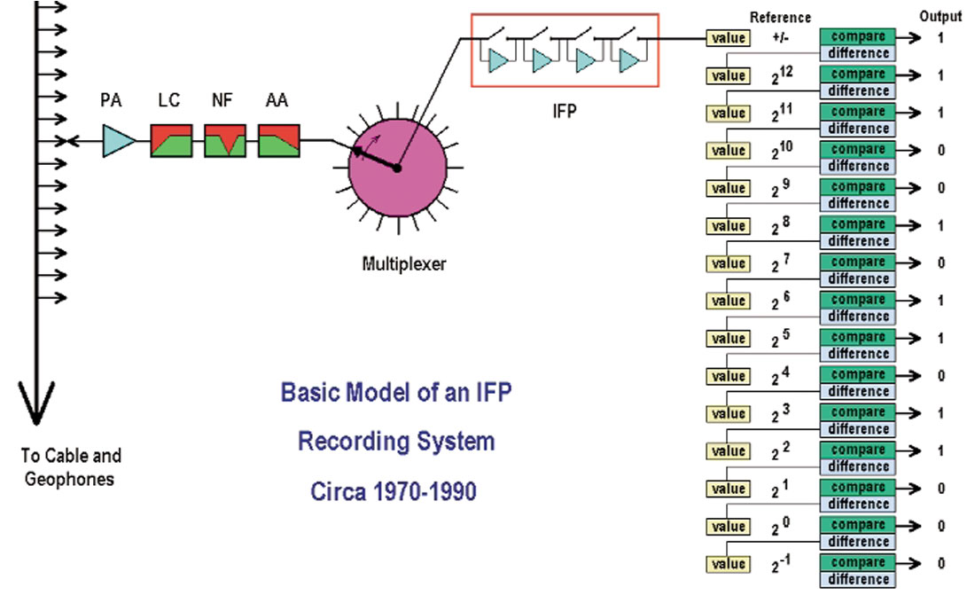
Upon entering the recording truck, the signal passed through “unscramblers” (a hard-wired cable link that picked off data from every Nth takeout) and was passed on to the “Roll-Along” switch. This switch allowed us to connect our recording instruments to some sub-set of the incoming channels. The signal for each recorded trace then passed through the pre-amplifier (“PA” in Figure 1) where it encountered common-mode rejection filters, surge protectors and a linear amplifier that provided a fixed gain selected by the operator (usually 24, 36 or 48 dB). The signal level was boosted to be strong relative to the electronic noise of our system and to put the average signal within the operating range of the rest of our system.
Next, the signal passed through a switch-selectable analog lowcut filter. In the later generation instruments, these filters could be selected with either an 18 or 36 dB/octave slope. The former had more phase stability but the latter was a more discriminating filter. One use of this filter was to de-emphasize the dominant low-frequency components of the incoming signal and therefore allow the instruments to be more sensitive to higher frequencies. The filter could be turned on or off and the slope altered by a simple switch on the panel of the instruments. Changing filter frequencies involved pulling the circuit boards out of the instruments and physically replacing one of the chips for each recording channel.
Another optional analog filter was the notch filter (denoted as “NF” in the diagram). This was sometimes used to suppress power line noise induced in our cables where they crossed or paralleled power transmission lines (or sometimes wire fences).
Since incoming data contained all frequencies of signal, we also required a high-cut, or anti-alias filter (labelled “AA” in Figure 1). This filter had to provide about 70 dB of attenuation at our digital sampling Nyquist frequency (250 Hz for 2 millisecond sample intervals). The steepest analog filter slope that could be engineered that remained stable over our range of operating conditions was 72 dB/octave. Therefore, this filter had to start its roll-off one octave below the Nyquist frequency (typically 125 Hz). In high-resolution data areas, we often employed an “extended” anti-alias filter of 180 Hz. This allowed some aliasing of data from 250-360 Hz, which could potentially distort data from 140-250 Hz. However, the extension of unfiltered data from 125 to 140 Hz was achieved.
All three analog filters were accused of instability, particularly with respect to the phase of the recorded signal. In fact, later generation instruments offered very stable filters given that a gentle slope was used and that the filters were frequently calibrated. Therefore, the low-cut filters were very stable (at 18 or 36 dB/octave). The antialias filters were near the limit of stability at 72 dB/octave and were usually active at frequencies beyond our recoverable signal bandwidth. The greatest offenders with respect to phase of the signal were the notch filters. Most geophysicists religiously avoided the use of these.
Next in our instrumentation sequence was a multiplexer – a rapid electronic switch that sampled all incoming channels once every sample interval. In a 120-channel DFS V, there were two analog modules, each servicing 60 channels. Each box had a multiplexer that would take a pulse of about 18 microseconds from one channel, leave a 15 microsecond gap, then move to the next channel. After 2000 microseconds (2 milliseconds), it would have sampled 60 channels and then be re-positioned to take the next sample from the first trace again. The output of the mulitiplexer was a slightly skewed (relative to time zero) set of sixty pulses representing one “scan” of all the channels followed by successive scans (one per sample interval) up to the recorded trace length. In other words, the multiplexer delivered a stream of discretely sampled pulses at the rate of about 30,000 pulses per second to the A-D converter. The multiplexer was another source of crossfeed, as well as being a source of harmonic distortion due to switching transients. The IFP amplifier and A-D converter that were downstream from the multiplexer had a limit of about 30,000 operations per second. Therefore, if we wanted to record 1 millisecond sample intervals, we were limited to 30 channels per analog module. Recordable channels were determined by our sample rate.
The Instantaneous Floating Point (or IFP) amplifier was next. Its job was to take each pulse delivered by the multiplexer and scale it to a voltage between approximately 4 and 8 volts. This would cause all of the bits of the following A-D converter to be exercised. Basically, the IFP amplifier consisted of four linear amplifiers that could be included in the signal path or bypassed by the closing of a transistor switch. If all four amplifiers were bypassed, a strong signal would receive no additional amplification. If all four amplifiers were activated, a weak signal could receive maximum amplification. The various combinations offered 24 dB of time-variant dynamic range. It is easy to imagine that the switches in this circuit were very active. They could change positions up to four times each sample or 120,000 times per second. The IFP amplifier was the greatest offender for harmonic distortion due to the high level of switching transients. The IFP amplifier contributed four “gain” bits to each recorded sample.
The scaled pulses were then passed to the Analog to Digital (A-D) converter. This device measured the amplitude of each pulse and formed a binary digital sequence of 15 bits to describe that amplitude. The type of device employed is known as a “Linear Successive Approximation Analog to Digital Converter”. The significance of the term “Linear” will be hilighted in the next section. “Successive Approximation” refers to the ladder-style configuration seen on the right side of Figure 1. In the most significant bit (at the top), the signal is compared to a DC threshhold to see if it is positive or negative. Then the rectified signal is then compared to a series of reference voltages. These are constant values presented by a high precision voltage generator and usually range from 212 millivolts (4.096 volts) at the most significant extreme down to 2-1 millivolts (0.0005 volts) at the least significant end. At each step, the incoming pulse voltage (“value”) is compared to the reference voltage. If the signal value is smaller than the reference, a binary “0” is written and the pulse flows down to the next step. If the signal value is larger than the reference, a binary “1” is written AND the pulse voltage is reduced by the magnitude of the reference voltage before passing as the value for the next step. The binary numbers shown in the diagram represent a pulse in the range of +6.50800 to +6.50849 volts.
The smallest non-zero value that could be represented was when the least significant bit was “1” and all other bits were “0”, representing a voltage of 0.0005 volts (or less). The largest value that could be represented was when all bits were driven to “1” which would occur for any voltage of 8.1915 volts (or greater). Therefore the dynamic range of this A-D converter was: 20 * LOG (8.1915 / 0.0005) = 84 dB. Since this device produced one binary number for every time sample of each trace, this was referred to as “Instantaneous Dynamic Range”. Remember that the IFP amplifier allowed the A-D converter to slide over a range of signals spanning 24 dB as time passed by. Plus there were three selectable pre-amp gain settings that could be changed from one prospect area to another (adding another 18 dB). Therefore, the total “System Dynamic Range” was quoted at 126 dB. However, can we see the weak 100 Hz component of the Swan Hills reef reflection at the same instant as its dominant 15 Hz component – or the strong noise at that time? This is a question of “Instantaneous Dynamic Range” which was limited to a theoretical 84 dB. In practise, all of the complex electronics in this system generated sufficient buzz and hiss (electronic noise) that we seldom realized more than about 66 - 72 dB of instantaneous dynamic range. The combined binary number written to tape for each sample was 2 1/2 bytes (20 bits) consisting of 4 gain bits, a sign bit, 14 bits of mantissa and a parity bit. Some systems would forego the parity bit and add one more bit to the mantissa, however this “extra” bit was usually dominated by instrument noise.
To summarize, then, the old IFP systems had several disadvantages (not necessarily in order of importance):
- Long analog signal transmission paths before digitization - subject to induction and distortion of signals
- Heavy cables not conducive to Heliportable or people-portable operations
- Channel to channel crossfeed in the cables
- Harmonic distortion in pre-amplifiers
- Amplitude and phase distortion of analogue filters
- Crossfeed and harmonic distortion from multiplexers
- Recordable channels limited by small sample intervals
- Switching transients and harmonic distortion due to IFP amplifier
- Transients due to Successive Approximation A-D converter
- Limited instantaneous dynamic range due to Successive Approximation A-D converter
- Large amount of electronics per channel requiring large power supplies
- Large amount of electronics generating substantial electronic noise relative to weak signals
Distributed Telemetry Systems
During the 1980’s various distributed telemetry systems emerged that allowed us to record more channels without enlarging our cables unrealistically. The instruments were packaged into small “boxes” and put close to the geophones. Depending on the system, there might have been one box to service each 8, 6, 3 or 1 geophone groups. Signals were digitised and conditioned in boxes distributed in the field near the geophones (shortened analog paths). The digital numbers were then relayed from box to box and were re-generated at full strength at each relay point (telemetry). Digital data transmission could be accomplished down a few pairs of wires, thus lightening cables and allowing very large active recording spreads.
At the same time, spread testing hardware and software was extensively developed, enabling us to identify poor geophone groups from the recording truck. Testing, analysis of impulse responses and reporting software has vastly changed the observer’s ability to identify poor geophone groups. Some software can often locate poorly planted geophones! It is easy to demonstrate that geophone coupling and overall quality of the geophone plants affects the quality of our recorded traces far more than just about anything else we do. Therefore, the ability to measure this parameter and to dispatch trouble shooters to repair bad sets is a huge advantage compared to our old style of operations and quality control. Today, we often record active 3D patches consisting of thousands of channels that may be distributed over hundreds of kilometers of line. Electronic monitoring of plant quality is vital in these programs. However, we must recognize that the automatic spread checking can only be effective if we use only a few geophones per group (nine or less). Within large groups, faults with individual geophones become very difficult to detect.
Early distributed telemetry systems utilized the same instrument topology as described in the previous section. Each box consisted of sufficient electronics to digitize a few channels. However each channel still used pre-amplifiers, analog filters, multiplexers, IFP amplifiers and successive approximation A-D converters. Therefore, complex electronic circuits were still used and power supply became a significant issue. Distributed telemetry systems were powered by batteries or solar panel – battery combinations. These may have been located sparsely along each receiver line (power-down-line systems) or, in some systems, required for each box. Either way, battery management became a big part of the job for field crews.
This generation of systems used a single data path to collect digital data. Data flowed from box to box along receiver lines to be collected by “Line Taps” (or “Crossing Station Units). Then a single control line or “backbone” was used to relay data from line to line across the survey to the central recording truck.
Throughout the 1980’s, then, we saw improvements due to the evolution of distributed telemetry systems and general improvements in control electronics:
— Shorter analog transmission paths
— Lighter cables for Heliportable and people-portable operations
— Reduced induction noise and crossfeed in the cables
Delta-Sigma (“24-Bit”) recording systems – a different tool
By the early 1990’s we began to use a different technology in large scale land acquisition tools. Most people know this technology as “24-bit” recording, although the correct name of the technology is “Delta-Sigma”. This was considered a “New Technology” to many of us who spent our lives with our noses buried in land seismic operations. However Delta-Sigma technology had been in common use in the music and recording industry for about 20 years. So called “Digital Streamers” had incorporated this tool for about 5 years in marine operations prior to the first land-based system being developed. Several small scale engineering systems had been in common use. However, the Delta-Sigma systems of the ‘70s and ‘80s were energy inefficient and required substantial power to run them. This made them poor candidates for large channel, land-based distributed telemetry recording systems. Developments in VLSI technology (Very Large Scale Integration) resulted in very small-wafer, low power-consumption systems being developed. In 1991, Input/Output sold their first production run of the I/O System Two recording system. Shortly thereafter, every major manufacturer was converting their lines to include Delta-Sigma technology. It has now become the standard of our industry
The Delta-Sigma modulator is at the heart of the technology. Its job is to produce a rapid stream of ones and zeros representing two voltages such that the average of the represented voltages converges to the input value. Figure 2 shows a simplified diagram of one channel.
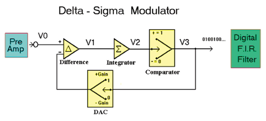
For our example in this paper, we will assume that the gain of the system is 10 volts (therefore a binary “1” represents +10 volts and a binary “0” represents –10 volts). The modulator is a chip circuit that operates on a 256,000 Hz clock (it will complete one cycle of operations for each clock cycle).
Now our signal comes along a short analog path to a preamplifier designed to set all signals to within the gain of the system. Next the signal is passed to a differencing op-amp (operational amplifier) where a feedback signal is subtracted (this signal will be + or – 10 volts depending on the previous clock cycle). The resulting difference is passed to an integrator that will add V1 to the previous voltage that occupied the integrator. A sign bit converter determines if the current signal in the integrator is positive or negative. If the current value in the integrator is positive, then a binary “1” is produced and passed out of the modulator. Also, the feedback loop is set to generate a positive 10 volt feedback, which will then be subtracted from the input next cycle. A negative voltage in the integrator generates a binary “0” and a negative 10 volts is generated for feedback. The stream of 1’s and 0’s is passed into the Finite Impulse Response (FIR) Filter. Remember each “1” is a code for +10 volts and each “0” is a code for –10 volts. A running average is formed. Each 2 milliseconds (512 clock cycles) the average is written as a full floating-point IEEE value. The following table shows the result of the first 15 cycles for a –3 volt input signal.
| Cycle Number |
Input Voltage V0 |
Difference Voltage V1 |
Integrated Voltage V2 |
1-Bit A/D |
Running Average |
|---|---|---|---|---|---|
| 0 | 0.00000 | 0.00000 | 0.00000 | 0 | 0.00000 |
| 1 | -3.00000 | -3.00000 | -3.00000 | -10 | -10.00000 |
| 2 | -3.00000 | 7.00000 | 4.00000 | +10 | 0.00000 |
| 3 | -3.00000 | -13.00000 | -9.00000 | -10 | -3.33333 |
| 4 | -3.00000 | 7.00000 | -2.00000 | -10 | -5.00000 |
| 5 | -3.00000 | 7.00000 | 5.00000 | +10 | -2.00000 |
| 6 | -3.00000 | -13.00000 | -8.00000 | -10 | -3.33333 |
| 7 | -3.00000 | 7.00000 | -1.00000 | -10 | -4.28571 |
| 8 | -3.00000 | 7.00000 | 6.00000 | +10 | -2.50000 |
| 9 | -3.00000 | -13.00000 | -7.00000 | -10 | -3.33333 |
| 10 | -3.00000 | 7.00000 | 0.00000 | +10 | -2.00000 |
| 11 | -3.00000 | -13.00000 | -13.00000 | -10 | -2.72727 |
| 12 | -3.00000 | 7.00000 | -6.00000 | -10 | -3.33333 |
| 13 | -3.00000 | 7.00000 | 1.00000 | +10 | -2.30769 |
| 14 | -3.00000 | -13.00000 | -12.00000 | -10 | -2.85714 |
| 15 | -3.00000 | 7.00000 | -5.00000 | -10 | -3.33333 |
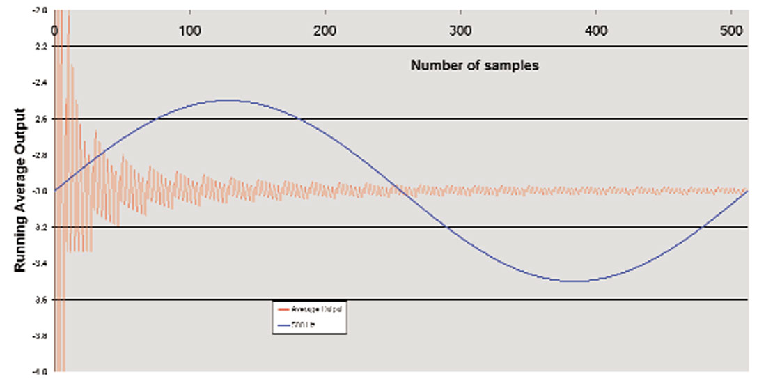
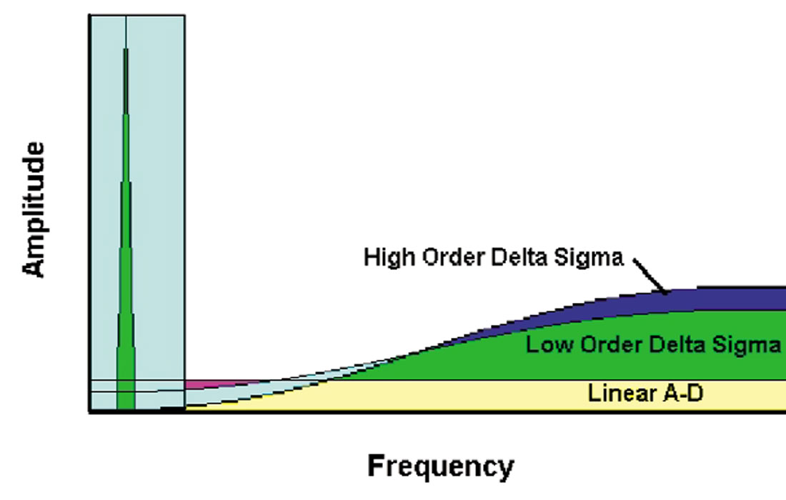
Figure 3 shows graphically the running average (red curve) for the first 512 cycles of a steady-state –3 volt input. Notice that the output converges to the input voltage but still exhibits a hashy noise about the exact value of –3. This noise is due to errors in our estimate of the signal and is called “Quantization Noise”. Recall that the modulator completes 512 cycles every 2 milliseconds. Therefore, a 500 Hz cosine would exhibit just one cycle in this same period of time. Obviously, the quantization noise is very high frequency. In fact it is dominantly 64,000 Hz to 128,000 Hz. The rapid sampling of this device gives us a very high sampling Nyquist frequency (128,000 Hz). Quantization noise is distributed over the bandwidth from 0 Hz to the sampling Nyquist. The fact that an integrator is included in the modulator renders this a non-linear device which results in the shaping of the quantization noise into very high frequencies (much like squeezing toothpaste in a half empty tube so one end is nearly empty while the other end is nearly full). By implementing higher order modulators (more integrators), we can exaggerate this noise-shaping characteristic (as seen in Figure 4). Having moved this noise into very high frequencies, we can now apply a digital filter to the binary sequence and eliminate all contributions above 200 Hz (for example). The result will be data in our desired seismic bandwidth that is free of quantization noise.
The Delta-Sigma system is a negative feedback device. When the value in the integrator becomes too large compared to the incoming signal, we apply feedback to reduce that value. When the value in the integrator is too small, we apply feedback that increases it. By measuring the average feedback, we can estimate the incoming value. If we over-sample greatly (take many many measurements), the average will have great precision.
The averaging, filtering and forming single high precision floating point numbers from the stream of 1’s and 0’s is the job of the FIR filter. If we request an output sample every 2 milliseconds, then 512 bits will be averaged and filtered. We will be 512 times over-sampled. The output sample Nyquist will be 250 Hz and the high-precision digital high cut filter must cut off below 250 Hz. If we request 1 millisecond output samples, then only 256 samples are averaged and we loose a bit of our precision. However, since each channel now has its own dedicated Delta-Sigma modulator, there is no need to reduce the channel capacity of the system when we record at 1 millisecond sample intervals. The output sample Nyquist will be 500 Hz and the digital high-cut must cut off below that (usually about 400 Hz).
The high cut filter is often called a “Brick Wall” filter. It is a high precision digital filter formed for the rapidly sampled data and has very stable characteristics. Basically the pass band is 100% up to within a few Hertz of the cut off. The cut off slope is extremely steep. With older analog anti-alias filters the slope had to be less than 72 dB/octave and data well back of the output Nyquist was filtered. This is no longer true and data can be trusted up to the cut-off of the high-cut filter.
The Delta-Sigma modulator is a compact circuit that generates negligible electronic noise. Most of the previous electronic analog circuits of the IFP system are eliminated to keep the noise floor very low. Only the pre-amplifier now precedes the modulator. This means not only reduced electronic noise, but also much reduced power requirements. Within the instruments the data path becomes digital without the interference of a lot of analog circuitry. Although the spectral shaping effect of low cut filters was desirable in the older systems, such a filter in the new systems would increase electronic noise to the point of undoing its own good.
The increased instantaneous dynamic range of these systems is sufficient that we no longer require the IFP amplifier to cover the full range of potential ground velocities. Therefore, we can dispense with the IFP amplifier. The circuits are relatively cheap to purchase and therefore it is affordable (and necessary) to dedicate one Delta- Sigma modulator with FIR filter to each channel. This eliminates the need for the multiplexer.
Today, the format of the written floating point number is IEEE (as opposed to the IBM format used in the past). This format bit shifts our data until the first bit of the mantissa is a binary “1”. The bit shift is transferred to the gain portion of the word. Since the first bit of the manitssa is now known to always be “1” it is not necessary to record it. Therefore we are free to record one more bit at the least significant end of the word. Thereby we gain 6 dB more precision (in amplitude, 3dB in power).
Delta-Sigma systems are robust, light weight, low power, and high-fidelity. By replacing older distributed telemetry systems with this new technology, we gain:
- No amplitude or phase distortion due to analogue circuits (other than the pre-amp)
- Hi-fidelity high-cut filters allow us to use data to about 80% of output Nyquist
- No crossfeed or harmonic distortion from multiplexers
- Recordable channels are not limited by changing sample intervals
- But note that small sample intervals reduce over-sampling and sacrifice resolution (dynamic range) and increase bit load on cables
- No switching transients or harmonic distortion due to IFP amplifier
- Small amount of electronics per channel requiring lower power
- Small amount of electronics generating very limited electronic noise relative to weak signals
- Lighter weight boxes for heliportable and people-portable operations (fewer flights to deploy equipment – lower operating costs)
Dynamic Range in a Dynamic Earth
You may notice that in the preceding section, I did not list “improved dynamic range” as one of the advantages of Delta-Sigma systems. Before we reach any conclusions, let’s consider the amplitude spectra for three theoretical reflections (depicted in Figure 5). Our reflection energy diminishes with time due to four energy loss mechanisms:
- Reflection and transmission losses through a layered earth
- Mode conversion at higher angles of incidence (assuming we are not interested in the shear waves)
- Spherical divergence (also known as geometric spreading)
- Absorption – a loss that effects high frequencies more than low frequencies.
The graphs in Figure 5 show the relative amplitudes for energy that is full amplitude at time zero, but is reduced by spherical divergence and absorption only. We have not attempted to account for reflection losses or mode conversion and longer offsets. In other research, we have calculated that for a linear increase in velocity, the average transmission loss may only be about 50 percent (-6 dB) after two seconds. In reality, transmission losses are much more strongly effected by locally variable geology.
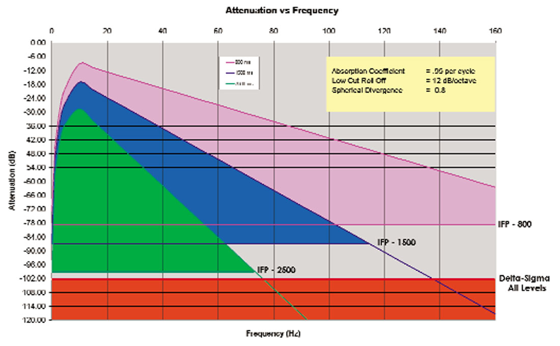
Spherical divergence was calculated using e-a•t where “a” was 0.8 and t is time in seconds. This represents the reduction of energy concentration as a wave front spreads out spherically from the source point. Absorption represents the energy lost per cycle of transmitted energy. This is generally regarded as losses to frictional energy and is probably dissipated as heat. An absorption coefficient of 0.95 was used in Figure 5, meaning that the absorption factor applied is 0.95f x t . In addition to these two factors we have added the effect of 10 Hz geophones with a 12 dB per octave roll-off. We have found these factors to be generally consistent with real-earth observations.
This yields the familiar observation that amplitudes of the high frequencies diminish more rapidly than for low frequencies and that this phenomenon is more exaggerated for deeper reflectors. Note that even the peak frequencies of each reflector diminish as depth increases.
This yields the familiar observation that amplitudes of the high frequencies diminish more rapidly than for low frequencies and that this phenomenon is more exaggerated for deeper reflectors. Note that even the peak frequencies of each reflector diminish as depth increases.
Let’s assume that if data with these characteristics was recorded by an older IFP system, that the IFP amplifier (together with an appropriate pre-amp gain) would have sufficient range to equalize the peak frequencies of each reflector as time passed. So 9 dB of gain might be applied to the 800 ms reflector, 17 dB to the 1500 ms reflector and 28 dB to the 2500 ms reflector. Then, as each of these reflections passed through the A-D converter, let’s assume that we could record an additional 70 dB of instantaneous dynamic range. We have marked the limit of recordable data for each reflector (79 dB, 87 dB and 98 dB respectively). Note that this results in an upper limit of recordable bandwidth of something in excess of 160 Hz for the shallow reflector, about 113 Hz for the medium reflector and about 73 Hz for the deep reflector. This analysis does not consider energy loss or coupling of geophones in the weathered layer. Buried geophone studies (where geophones are cemented some 20 meters below the surface) have shown that the results in Figure 5 are realistically obtainable in favorable areas. (Weathering layer effects probably act mostly as an additional high-cut filter and may not affect the shape of these curves below a certain frequency. The high-cut frequency would be area dependent, but is often in the 90 to 120 hz range with a modest slope. The preceding sentences in brackets are speculation on the part of the author based on casual observation of many field tests.)
Bench tests performed by Tim Hladuk of Geo-X for a 1992 presentation co-authored by Tim and myself, indicated the realizable dynamic range of Delta-Sigma systems was probably in the order of 100-110 dB depending on the harmonic distortion of the pre-amplifiers. We have marked this limit as a red bar across the bottom of Figure 5.
The Delta-Sigma dynamic range appears as a fixed limit since there is no IFP amplifier to change gain settings as time passes. Note that we have not gained any significant dynamic range for the deepest reflector compared to the IFP system. However, for shallower reflectors, the Delta-Sigma system certainly offers more accessible dynamic range and very likely should allow us to record more bandwidth. We should be very careful with statements that claim modern systems have more dynamic range. In fact, we have exchanged a two stage system consisting of instantaneous dynamic range (limited by a successive approximation A-D converter) plus time variant dynamic range (offered by an IFP amplifier); and we now have a system which delivers all its dynamic range instantaneously. There will be situations where we may realize an improvement in total dynamic range, and there are certainly situations where we may not.
Regarding dynamic range then:
- We have exchanged about 80 dB of instantaneous dynamic range, plus about 24 dB of time variant dynamic range for about 100 dB of all instantaneous dynamic range.
- This means that we can expect some realizable gains due increased dynamic range in shallower reflections,
- But perhaps we will not realize very much improvement for deeper reflections.
Noise, Processing and Precision
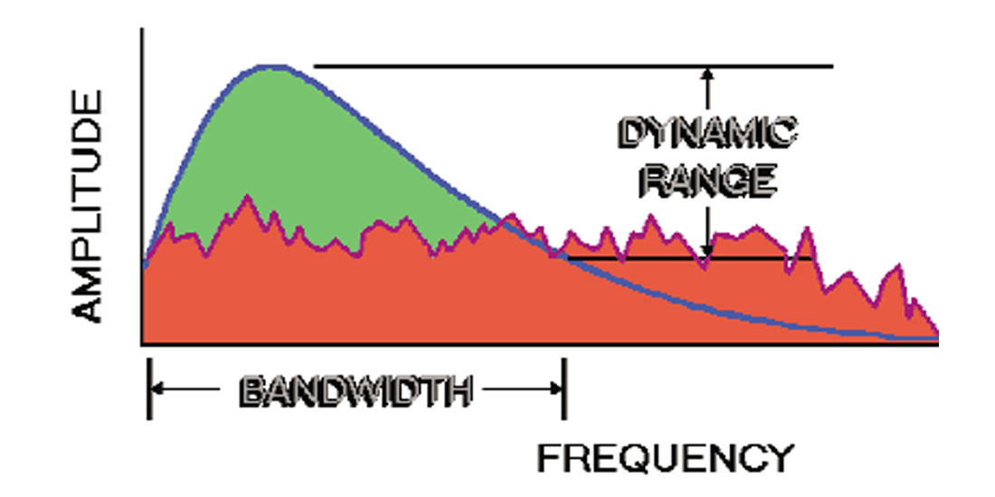
Figure 6 shows a generalized amplitude spectrum for recorded field data. We have intentionally omitted all scales as actual values will vary greatly from prospect to prospect. The blue curve indicates a signal spectrum affected by low-cut filters of geophones and instruments and a high-cut due primarily to earth absorption (proportional to a 1/x curve when plotted on a linear amplitude scale). The red, hashy area is intended to represent various forms of noise. Some elements that could contribute to noise include (not necessarily in order of importance):
- Quantization noise
- Electronic noise and harmonic distortion from instruments, cables and geophones
- Time variant random noise (traffic or wind on the spread)
- Offset dependent, source generated noise (ground roll, air blast, trapped mode)
- Source dependent noise (SP’s in muskeg or sand versus on hard surfaces)
- Receiver dependent noise (stations near pump jack, or under power line)
- Spatial aliasing (from using large group intervals without geophone arrays)
- Operational noise (poor geophone plants, poor quality control)
The fact is that dynamic range of our instruments is seldom the limiting factor in recoverable bandwidth. More often, we are limited by our ability to see through noise. One of our most common defences against noise is CDP stacking. But we must realize that even a 64-fold stack will provide only 8 times signal to noise improvement – and then only under the ideal assumption of identical signal on each trace and Gaussian distributed, random noise on each trace (conditions seldom consistent with real data). An improvement by a factor of 8 translates to an 18 dB gain of signal against noise. If we start with a signal to noise ratio of 1:1, then 18 dB suppression of noise after stack does not offer very much dynamic range! From another perspective, let’s assume that our instruments offer only 100 dB of dynamic range and that our noise floor is 82 dB below maximum signal. Then a perfect 64 fold stack will just drop the noise floor to the limit of the instruments. Now, how often is our noise 82 dB below our peak signal? Not very often! Therefore, recorded noise is usually our current limit of dynamic range.
One factor in dynamic range that is not usually considered is the numerical precision of our processing algorithms (particularly the FFT). Every filter, every deconvolution, and many operations in processing use the FFT. And yet it has been demonstrated (“Update of Land Seismic Acquisition Tools and Techniques” – paper presented by Norm Cooper, CSEG Convention, May 2002) that the numerical round-off error in these algorithms accumulates to an effective noise level at about –100 dB and that poorer implementations of the algorithm can result in noise up to –80 dB. Ask any processor just how effective his deconvolutions are, how deep into the data can they reach and recover useable signal and the response is seldom more than “about 40-60 dB”.
It seems that our greatest limit regarding useable data is tied to the level of noise in our data much more than to the dynamic range of instruments. To gain more from our data, we must develop more powerful methods and algorithms to manage noise. The old assumptions that noise is random are inappropriate. Perhaps we can focus more on some methods that have been tested using deterministic methods of noise analysis and removal. Why don’t we delay the time break of each shot by one second so we can record a 1 second estimate of noise at each geophone location for each shot? Certainly, we must do all in our power to reduce the noise generating factors identified at the beginning of this section.
Now What ???
Current developments in instrumentation continue to improve dynamic range, reduce system weight and power consumption, expand channel capacity and strengthen operational factors. Modern distributed telemetry systems are network based nodal systems with multiple and redundant data paths. This means that a cable break along one control line will not cease operations.
Many instrumentation developments have been, and will continue to be, targeted at obtaining more data, more efficiently and at lower cost (examples include, lighter cables and boxes, reducing per-box or per-channel manufacturing costs, improving reliability to reduce maintenance costs, adding data path redundancy to reduce down-time). Other developments are targeted at improving recorded data quality (examples would include the use of marsh cases and planting poles for geophones, development of highly diagnostic spread checking software, re-engineering of preamps to reduce harmonic distortion, shortening analog data paths).
One of the more recent developments includes I/O’s “Vectorseis” system. One aspect of this system is that it conveniently and accurately obtains 3-component data. However, there are many other appealing attributes. This is a digital sensor (based on Delta-Sigma concepts) with no analog data path. It has a level impulse response down to (or nearly to) zero Hz (no low-cut roll off). The technology may be capable of delivering dynamic range of about 160 dB. But perhaps one of the greatest benefits is that it comes in a tubular package that forces us to drill holes into the near-surface earth and couple the sensor in these holes. If my speculation in a previous section is correct, then perhaps this is a start at overcoming the earth’s exaggerated high-cut filter due to the weathering layer and coupling. Methods developed by Veritas Geophysical have resulted in high field productivity (averaging about 1000 stations picked up and laid out each day).
We must maintain continued development in processing with a focus on signal to noise enhancement algorithms and numerical precision. Accuracy and turn-around time are both important, but perhaps we could use one generation of computer speed improvement to focus on increased numerical accuracy rather than increased turn-around time (for example: maintaining higher precision numbers, using double padding of FFT’s, exploring alternate transforms, researching and developing other numerical methods that are beyond this author’s grasp)
Summary
It is very important that we continue to evolve systems and methods that enhance data quality and increase system performance. We must not use gains in one area to justify poor practices in another area. To this end, we offer the following thoughts and objectives (many of these introduce concepts not addressed in this article, but we feel they are all part of optimizing signal and minimizing noise within our useable dynamic range):
- Continue to shorten or eliminate analog data paths
- Increase system dynamic range (not just in acquisition, but also in processing)
- Reduce power consumption, harmonic distortion and weight either by simplifying electronics or by shrinking them (VLSI, MEMMS)
- Enhance sensor coupling by developing efficient containers and field methods
- Continue development of automated sensor testing and quality control to optimize quality of field operations
- Use sufficiently small group intervals for discretely sampled spatial data (grouped or single sensors)
- Use analog geophone arrays to reduce aliased noise if larger group intervals must be considered
- Optimize coupling of energy source by recognizing effects of the inelastic zone and coupling versus charge size in dynamite (i.e. do not use charges far in excess of those necessary to generate sufficient reflection energy at desired offsets, consider using several distributed small charges rather than single large charges)
- Optimize coupling of energy source by recognizing hold down weight versus harmonic distortion in Vibroseis (i.e. do not exceed 65 to 70 per cent drive levels)
- Allow line deviation within realistic tolerances in order to seek areas of better source and receiver coupling
- Understand statistical noise introduced by survey design and irregular offset (and azimuth) sampling, ensure that your designs are sufficient considering the signal and noise characteristics of your prospect area
- Choose a sample interval appropriate to your realistic estimate of recoverable bandwidth (consider up to 80% of output sample rate Nyquist as reliable). Recording smaller than necessary sample intervals will reduce dynamic range and precision and will increase bit load on digital telemetry circuits (potentially increasing acquisition time and costs).
- Don’t expect dynamic range of instrumentation to compensate for poor choices in other parameter selection. Increased dynamic range will only be useful to us provided we fill the extra range with signal, not noise!
We must all be aware of the tools of our trade and not succumb to the fate of the old Swedish logger. You may remember the story of the hardworking wood-cutter who disappeared into the forest each day with a large, sharp hand saw. He would return each night having cut and stacked 1.5 cords of wood. One day, a young salesman introduced the old Swede to a new tool, the “chain saw”. The old man was sceptical of the new tool, but the the salesman assured the woodsman that he would triple or quadruple his output with this great new invention. After three days of exceedingly hard work, the exhausted worker returned the saw to the salesman. “I’ve tried my hardest …” he said, “… but I can’t get more than a cord a day with this contraption. I’m afraid it just doesn’t work as well as you claimed!”
The young man looked puzzled and took the saw. “There must be something not adjusted correctly“ he stated. “Let me try it out.” And he started the gas engine with no difficulty. The surprised Swede jumped back and shouted “What’s all that noise?”
Given an ever changing set of tools, we must be sure we understand their power as well as how and when to apply them. Without this understanding, we will be disappointed and overworked, indeed.


Join the Conversation
Interested in starting, or contributing to a conversation about an article or issue of the RECORDER? Join our CSEG LinkedIn Group.
Share This Article