Let us be straight with one another. Well, perhaps more to the point, let us be sinusoidal with one another. Communication is key in every industry. The words and images that are being used in this article are an attempt at modeling my thoughts in order to transmit them to you for your consideration, response or refinement. As a group we more or less speak the same language and, due to sharing a similar culture, the words employed elicit more or less the same mental images. Iay ancay enevay codeenay omesay foay ethay ordsway danay ouyay ancay opecay. Granted, the communication would have been aided greatly had I given accurate forewarning of the encoding used in the previous sentence. However, more than likely you looked at the ‘words’, identified the situation and adapted. If inaccurate forewarning had been provided communication would have suffered even more .
Although sometimes huge, the seismic data file in SEGY format is one of the key components or ‘words’ of our industry communication. These files represent ‘words’ passed around within the milieu of processors, data-loading specialists, interpreters, partners, brokers and service providers. These ‘words’ are encoded, however is it not a compulsory encoding. Fortunately, the culture has adapted to cope with certain variations. One of the more subtle and hence dangerous problems is floating point data sample misrepresentation and it is the one that I would like to highlight in this article.
I will restrict the discussion to two ways of encoding floating point values. The first is the IBM single precision floating point (‘ibm’) and the second is the ANSI/IEEE Std 754 - l985, or IEEE 4 byte floating point (‘ieee’). The 1975 SEG standard for SEGY format describes the use of ‘ibm’ for re p resenting floating point seismic samples. The forewarning (data sample format code) about the encoding is contained in a word location in the binary header (byte 25-26) and a value of ‘1’ indicates that floating point representation is being used for the data samples. There is no mention of the ‘ieee’ representation which was not formalized until ten years later. In the interim, I believe, the CSEG SEGY committee proposed (date unknown, sorry) the use of ‘ieee’ for data sample representation with a data sample format code of ‘6’. The 2002 Rev 1.0 SEG Standard for SEGY Data Exchange Format deals with ‘ibm’ as before and has added ‘ieee’ and given it a data sample format code of ‘5’. Good, problem solved, let this stuff slink back to the esoteric realm where it belongs.
Not quite yet and it is highly unlikely the problem has been solved. It will be some time before Rev 1.0 trickle-down takes place and even so there is no systemic compulsion to change the data sample format code even if the numeric format (‘ibm’- to-’ieee’ or ‘ieee’-to-’ibm’) of the data samples is changed. The data sample format code, although in the same file, is relatively remote from the traces containing the data samples. Prior to 2002 there was no firm definition of what to change it to anyway. The majority of computer systems in use, since 1975, have adopted the ‘ieee’ as the native way of working with floating point. Many of the data files were changed to be store d on the working computers in this numeric format. It is unlikely that as many corresponding data format codes were also changed. As these modified files, instead of those rigidly following the data exchange format, were used as ‘words’, and passed around, the situation developed that either ‘ibm’ or ‘ieee’ data samples were or can be handled correctly or either were or can be mistaken for the other. Floating point confusion is one of the difficult problems with seismic data. This is irrespective of the arguments whether single floating point representations are an adequate model of the real number system or whether complier optimization routines properly handle floating point (see references). Even the more discussed ‘endian’ or ‘byte order of the data’ issue is not that dangerous as the result of confusion in that area is blatantly obvious. However, there definitely are instances of interpreters using SEGY data misrepresented through ‘ibm’/’ieee’ confusion, or derivatives of such data.
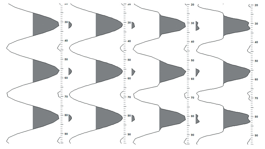
As you did in the first paragraph, we should look at what is displayed and learn to identify the situation first. The left portion of Figure 1 represents seismic data stored in ‘ieee’ format for the data samples as it was read in and displayed with no error. The middle and right portions represent the same data read in and erroneously displayed as ‘ibm’, and as ‘ibm’ with a display gain, respectively. The gain was applied to adjust to a similar view as that in the left portion. Figure 2 is a similar layout but the seismic data was stored in ‘ibm’ and erroneously displayed as ‘ieee’.
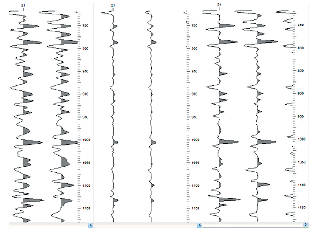
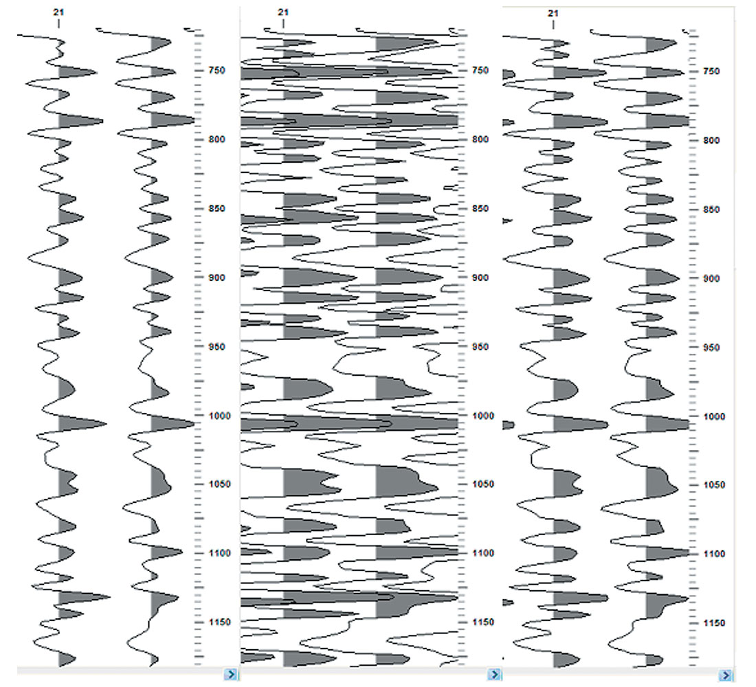
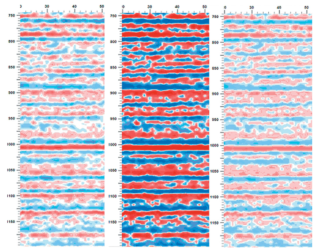
In both case above, depending on time pressures and or lack of direct involvement with loading or working up the data, the variable area displays are easy enough to slip by an interpreter. The panel on the right (‘‘ibm’ as ‘ieee’’), in Figure 2, seems to have lost the sinusoidal nature of seismic data and is perhaps the clearest example of the insidious nature of the problem. It is not difficult to imagine work situations that would make it extremely difficult or impossible to identify the data as containing bad values. Low resolution displays come to mind easily. Similarly, the variable density displays of misrepresented data, presented in a similar format in the middle and right panels of Figure 3 and Figure 4, after gain adjustment, are difficult to distinguish from the correct data in the left panels, other than the feeling of amplitude imbalance. Figures 3 and 4 were plotted with a relatively simple colour spectrum representing the amplitudes. Some of the more complex colour spectrums in use today may serve to highlight the problem or to further hide the problem. Personal experimentation with your favorite displays may shed some light on that question.

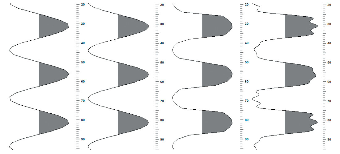
Visual discrimination or problem identification in the popular displays is probably the most important aspect to take away from this article. However, what is not shown by these displays is very disturbing. Other ways of looking at the data should be used. The majority of seismic variable area displays linearly connect the samples; additionally, under zoomed-in conditions, some displays may apply some form of parabolic smoothing function for a more pleasing look. Variable area colour smoothing has the same result of smoothing out the effects of the problem. The damage to the underlying signal is done and the displays are helping to hide the beast. A zoomed-view of the wave shape or its mutation is also instructive. A single frequency, consistent amplitude SEGY was created for Figures 5 and 6. The left-most panel of each figure shows the linear connection of the data samples of good data. The left central portion is after the signal is taken into the frequency domain, the number of cells increased by an amount to fill the displayed area, brought back to time, and displayed in the same way. It is ‘oversampled’. The right central panel shows the problem data, while the right-most shows the oversampled version of this. ( Maybe this should be called the Bart Simpson at rest effect?) The frequency is 42 hertz and amplitude was +/- 25000. No additional display amplitude scaling was needed to compare the waveforms.
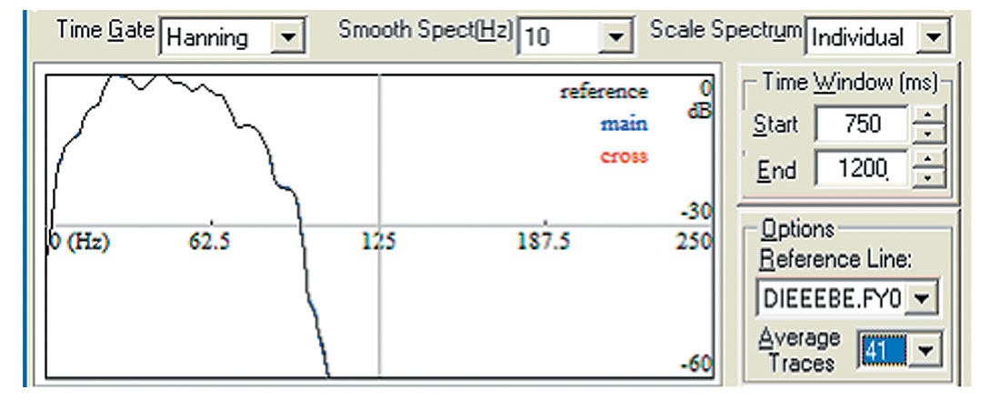
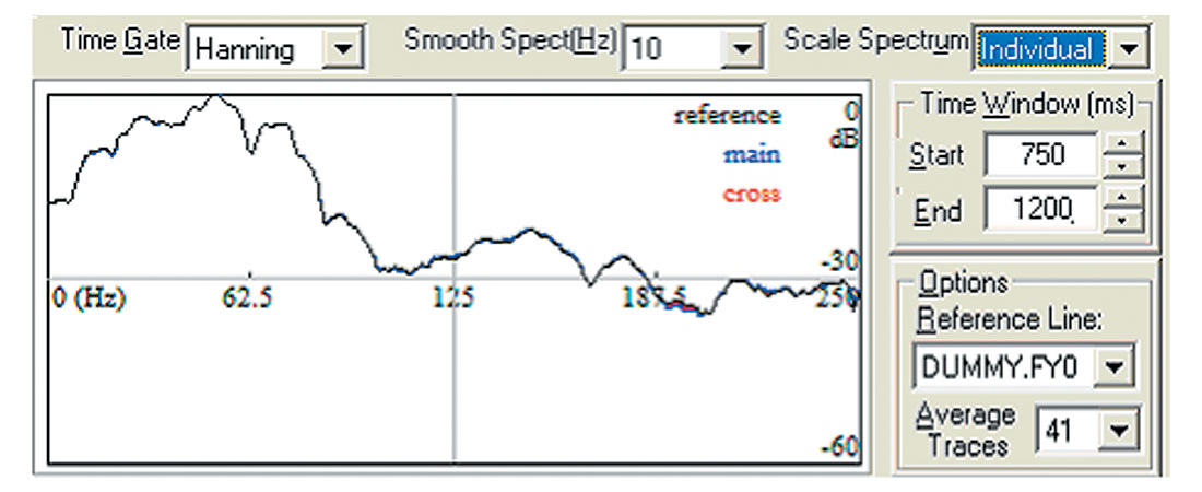
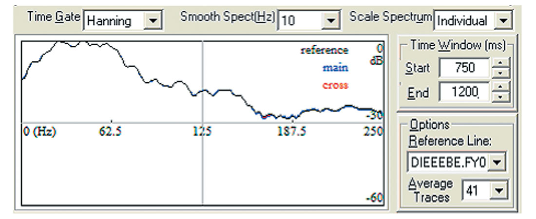
There is definitely something else living in there! Is there another measure? Reverting back to the original data file, in both error cases, Figure 8 and Figure 9 show no roll off of the noise at high frequencies with the problem data. The inappropriate response would be to filter it further and give the beast yet another cloak, but it is very tempting. As modern processing is evolving to a whiter spectrum this contamination becomes critical and perhaps the problem becomes harder to identify. Figure 7, represents the power spectrum of the ‘ieee’ data when properly dealt with. The good ‘ibm’ file exhibited a similar power spectrum and is not shown.
The base cause of the problem is that the bit positions defined by the two numeric formats of floating point samples (‘ibm’ and ‘ieee’) and the interpretation of these bits are different but not different enough to cause a blatantly obvious error. If you are not certain what you are looking for it is hard to spot the charlatan. To investigate a very specific example, let us take the floating point number encoded in the four bytes represented by the string of hexadecimal characters (talk about esoteric):
42 6C AD 15
To correspond with the charts below, 42 is byte 1, 6C is byte 2, A D is byte 3 and 15 is byte 4. This can be represented as 32 bits in a binary presentation:
Bit 1 - 0 1 0 0 0 0 1 0 0 1 1 0 1 1 0 0 1 0 1 0 1 1 0 1 0 0 0 1 0 1 0 1 - Bit 32
For those of you who type with more than two fingers, I would like to pause and review just a little about binary numbers. What is referred to as the ‘sign bit’ can be identified in the chart below but generally contains a ‘0’ if the number or mantissa is positive, or a ‘1’ if negative. As we are considering floating point numbers we would expect to find an exponent and a mantissa in there and the charts below show us where these are for the ‘ibm’ and ‘ieee’. In general the ‘MSB’ or most significant bit is on the left of the mantissa and exponent. Most significant? Would you rather win 1000000 in a lottery or 0000001?
There is no sign bit or binary point for the exponent as it is store d as a positive offset biased number. Explanation: if you are a bit stingy (pun) and want to re p resent -127 to 128 store it as 0 to 255 and pretend 128 is really 0. In both formats considered here the mantissa is really a fraction that will be multiplied by the sign and exponent. The unseen ‘binary point’ is considered to be left of the most significant Q bit (Q-1), in both cases. However, in the ‘ieee’ definition, there is assumed to be a 1 implied to the left of the ‘binary point’. The examples after each chart describe binary fractions which are a lot like decimal fractions, once you take time to think about it, so I will avoid that for now.
The charts, presented below, for the ‘ibm’ and ‘ieee’ representations were taken from the SEGY Rev 1.0 document.
IBM Single Precision Floating Point. (1975 - Code 1 and Rev1.0 May 2002 - Code 1)
4-byte hexadecimal exponent data (i.e. IBM single precision floating point)
| Bit | 0 | 1 | 2 | 3 | 4 | 5 | 6 | 7 |
|---|---|---|---|---|---|---|---|---|
| Byte 1 | S | C6 | C5 | C4 | C3 | C2 | C1 | C0 |
| Byte 2 | Q -1 | Q -2 | Q -3 | Q -4 | Q -5 | Q -6 | Q -7 | Q -8 |
| Byte 3 | Q -1 | Q -10 | Q -11 | Q -12 | Q -13 | Q -14 | Q -15 | Q -16 |
| Byte 4 | Q -17 | Q -18 | Q -19 | Q -20 | Q -21 | Q -22 | Q -23 | 0 |
S = sign bit. — (One = negative number).
C = excess 64 hexadecimal exponent. — This is a binary exponent of 16. The exponent has been biased by 64 such that it represents 16(ccccccc-64) where CCCCCCC can assume values from 0 to 127.
Q1-23 = magnitude fraction. — This is a 23-bit positive binary fraction (i.e., the number system is sign and magnitude). The radix point is to the left of the most significant bit (Q-1) with the MSB being defined as 2-1. The sign and fraction can assume values from (1- 2-23 to -1 + 2-23). It must always be written as a hexadecimal left justified number. If this fraction is zero, the sign and exponent must also be zero (i.e., the entire word is zero.) Note that bit 7 of Byte 4 must be zero in order to guarantee the uniqueness of the start of scan.
Value = S.QQQQ,QQQQ,QQQQ,QQQQ,QQQQ,QQQ x 16(ccccccc-64)
So let us see what the ‘ibm’ interpretation of our string of 4 bytes (42 6C AD 15 ) is:
Sign bit 0 so it is a positive value -10 = 1
Exponent is 1000010 binary or 66 decimal, so (ccccccc – 64) = (66- 64) = 2, giving 162 or 256
Mantissa: (bytes 2 through 4 less the last bit, which is not defined for ‘ibm’
Binary: 0 1 1 0 1 1 0 0 1 0 1 0 1 1 0 1 0 0 0 1 0 1 0 1
The MSB (left most) is valued at 2-1 or 1/2 , the second 2-2 or 1/4, through to the second from the last valued at 2-23 or 1/8388607.
If there is a one in the binary place you add the value of that bit to the total value of the mantissa. Hence the value of the mantissa is:
Q = 2-2 + 2-3 + 2-5 + … + 2-22 or Q = 1780549/4194304 = 0.424510
Hence the ‘ibm’ floating point value represented is + 0.42425 X 256 = 108.676
4-byte, IEEE Floating Point (1975 Standard Code N/A and Rev 1.0 May 2002 Standard Code 5
| Bit | 0 | 1 | 2 | 3 | 4 | 5 | 6 | 7 |
|---|---|---|---|---|---|---|---|---|
| Byte 1 | S | C7 | C6 | C5 | C4 | C3 | C2 | C1 |
| Byte 2 | C0 | Q -1 | Q -2 | Q -3 | Q -4 | Q -5 | Q -6 | Q -7 |
| Byte 3 | Q -8 | Q -9 | Q -10 | Q -11 | Q -12 | Q -13 | Q -14 | Q -15 |
| Byte 4 | Q -16 | Q -17 | Q -18 | Q -19 | Q -20 | Q -21 | Q -22 | Q -23 (Note 1) |
The value (v) of a floating-point number represented in this format is determined as follows:
| if e = 255 & f = 0. .v = NaN | Not-a-Number (see Note 2) |
| if e = 255 & f = 0. .v = (-1)s * • | Overflow |
| 0 < e < 255. . . .v = (-1)s * 2e -127 * ( 1 . f ) | Normalized |
| if e = 0 & f ? 0. . .v = (-1)s * 2e -126 * ( 0 . f ) | Denormalized |
| if e = 0 & f = O. . .v = (-1)s * 0 | ± zero |
| where | e = binary value of all C’s (exponent) f = binary value of all Q’s (fraction) |
NOTES:
- Bit 7 of byte 4 must be zero to guarantee uniqueness of the start of scan in the Multiplexed format (0058). It may be non zero in the demultiplexed format (8058).
- A Not-a-Number (NaN) is interpreted as an invalid number. All other numbers are valid and interpreted as described above.
And what would be the ‘ieee’ interpretation of our string of 4 bytes ( 42 6C AD 15 )? :
Sign bit 0 so it is a positive value -10 = 1
Exponent is 10000100 binary or 132 decimal, so (cccccccc – 127) = (132-127) = 5, giving 25 or 32
Mantissa: (bytes 2 less the first bit and bytes 3 and 4
Binary: 1 1 0 1 1 0 0 1 0 1 0 1 1 0 1 0 0 0 1 0 1 0 1
The MSB (left most) is valued at 2-1 or 1/2 , the second 2-2 or 1/4, through to the second from the last valued at 2-23 or 1/8388607.
Q = 2-1 + 2-2 + 2-4 + … + 2-23 or Q = 7122197/8388607 = 0.84903210 but we have to add the implied 1.
Hence the floating point value re p resented is + 1.849032 X 32 = 59.169
What is the right answer, 108.676 or 59.169? The answer is not determinable from the data samples alone, nor even from the data traces without some risky assumptions. The answer depends on the value of the data sample format code contents which at best was not rich enough to distinguish the formats from 1975 to 2002 and at worst may not be updated, on a format change anyway. To be fair, the 1975 standard defines a data exchange format and the ‘contract’ is not valid should we exchange files of any other description. It is my experience that all exchange is not under contract.
In this small SEGY sample file used there were 874500 such samples. The values that they represent range significantly in amplitude. The shift of the most significant bits of the mantissa to the exponent in the misinterpretation of ‘‘ibm’ as ‘ieee’’ and the reverse in the ‘‘ieee’ as ‘ibm’’ situation is only part of the problem. Depending on the bit pattern and amplitude, the effects change, making the problem very erratic and unpredictable. Detection of the condition and understanding what causes the problem should help. A long term solution may be better served if the Standard s Committee discuss a self defining element to the numeric format. Instead of being remotely identified, the trace could be self-identifying if the first element was given a guaranteed value. This would be similar to the Log Ascii Standard Committee (LAS) adoption of -999.99 as a null value. If something like -9 were used as the first sample value, any software working with this file could key on this sample, identify the numeric format (not to mention the byte order) and then ignore this sample unless it was added back in to write out the trace data. This would ensure that the descriptor is written out in the same numeric as the trace as a matter of standard practice. A data cost of 573/875073 or 0.065% would have been a small price to pay for peace of mind.
With access to an uncontaminated data file then it is certainly possible fix the problem by reloading it properly. If you do not have that chance because the problem was introduced historically and you do not have access to a good copy there is little that can be done to back out of the problem.
My advice in regard to this problem is similar to that given to a buddy who was going to drive with his family through the U.S., Mexico and down to Panama to open a Bed & Breakfast. Safety never sleeps.


Join the Conversation
Interested in starting, or contributing to a conversation about an article or issue of the RECORDER? Join our CSEG LinkedIn Group.
Share This Article