Rock Physics Template (RPT) Technology for Reservoir Characterization and 4D Seismic Monitoring

This paper describes the use of Rock Physics Templates (Avseth et al. 2005) in both reservoir characterization and 4D seismic reservoir monitoring. A major challenge in seismic exploration is the mapping of type, location and extent of hydrocarbon fluids. During reservoir production monitoring, the aim is to follow the temporal variations in the spatial distributions of fluids and changes during the production phase (Johansen et al. 2002).

Both static and dynamic rock physics template (RPT) analyses were performed on data in which gas sands were encountered in the well. The reservoir sandstone (zone of interest is between 2400-2530 m, Figure 1) is unconsolidated with some cementation. For this reason, friable sand (based on Contact Theory, CT) and constant-cement models (CCT) were tested on the dataset. In addition, a patchy cemented sandstone model was applied on the same dataset. The volume of cement considered during modeling was 3%; a shear friction factor of 0.3 was also used.

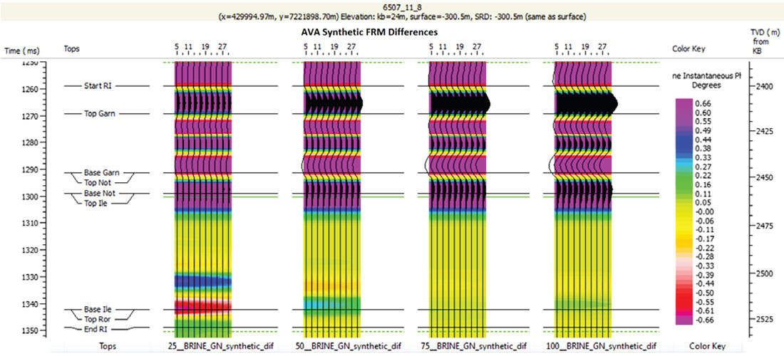
Gassmann’s fluid substitution modeling was applied to real log data to model 4D effects; the data included compressional and shear velocity logs, density logs to produce synthetic well-logs representing the reservoir at 25%, 50%, 75%, and 100% fluid saturations of brine and gas. The original and fluid substituted logs were used to compute amplitude versus angle (AVA) synthetics using Zoeppritz equations for near angle (5 degrees) and far angle (30 degrees), with a zero phase Ricker wavelet of assumed dominant frequency 25 Hz. Seismic amplitude variation on the computed AVA prestack synthetics shown as gathers was found to be successful at revealing brine substitution effects.

Figure 1 shows the original log data used in this analysis; these include gamma ray, volumetric, porosity, neutron porosity, density, saturation, resistivity, P- and S-wave and others.

Fluid-lithology detection and discrimination using P- and S-wave velocity cross-plot

During reservoir characterization, it is important to first discriminate between fluids and lithology. This was done through cross-plotting by combining P- and S-wave velocities and density. P- and S-wave velocity information is a good direct hydrocarbon detection method.

In spite of the many competing parameters that influence velocities, the non-fluid effects on P- and S-wave velocities are similar (Avseth et al., 2005). Variations in porosity, shaliness, and pore pressure move the data up and down along the same trend, while changes in fluid saturation move data from one trend to another (Avseth et al., 2005) allowing determination of which formations contain hydrocarbons as illustrated in Figure 2.

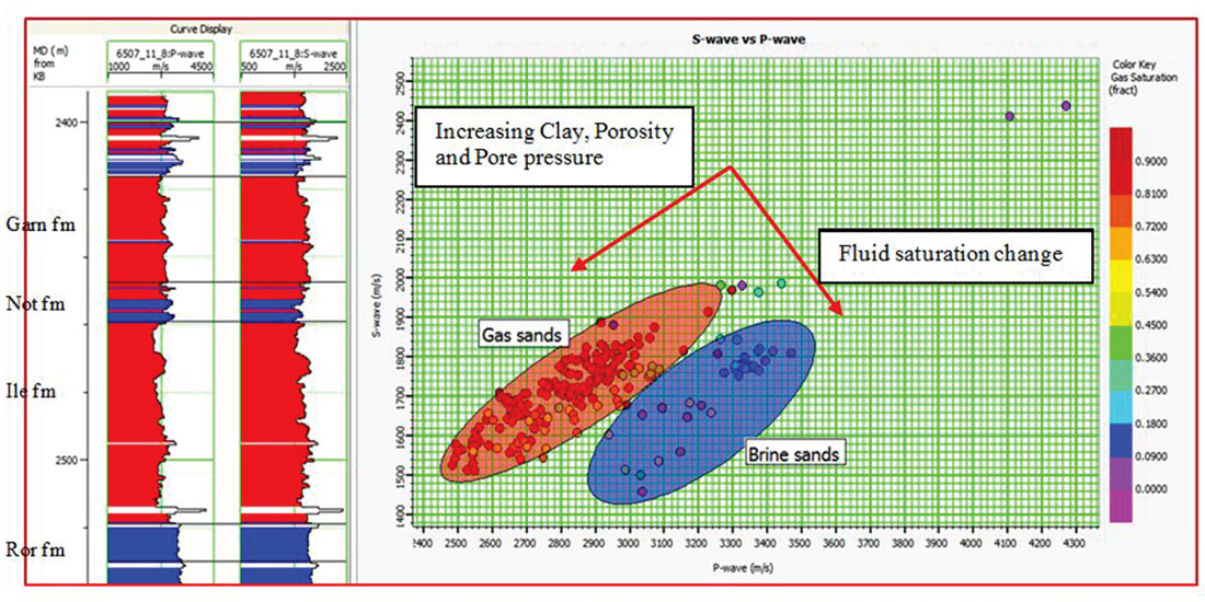
The cross-plot points in Figure 2 are color-coded using the gas saturation log; the P- and S-wave logs (in curve display) are color-coded based on the two zones (gas and brine sands) defined in the cross-plot domain. These two distinct zones of data are separated along the fluid saturation change trend. The data in the red zone represents gas sands, that in the blue zone represents brine sands. By projecting cross-plot zones to the logs, it becomes clear that gas is found in Garn and Ile formations whereas brine is in the Ror formation and some in the Not formation.

Reservoir characterization using a Rock Physics Template

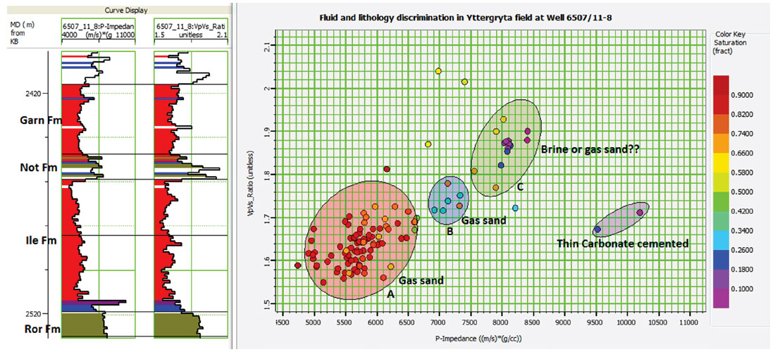
After successful discrimination between fluids and lithology as demonstrated in Figure 2, reservoir characterization was performed using Vp/ Vs versus AI, cross-plots to identify three main zones (A, B and C) as shown in Figure 3. Gas and brine sands have been identified and mapped on their corresponding reservoir positions. Thin Carbonate cemented sands are also visible at the base of Ile formation and on the cross-plot domain.

Reservoir characterization of data using a static RPT based on constant cement model

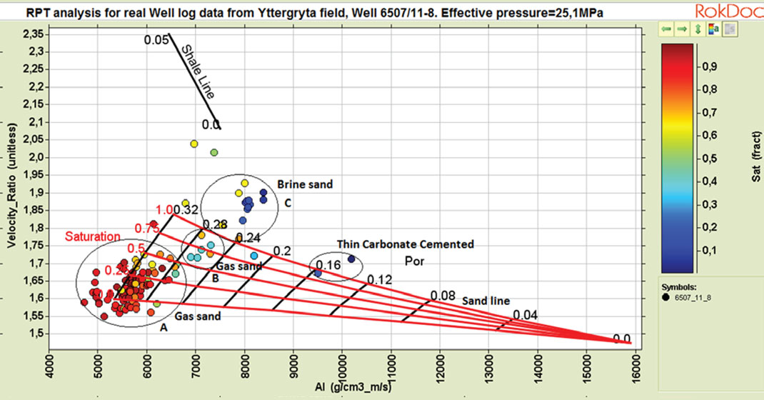
A constant-cement model was then superimposed on the Vp/Vs versus AI cross-plot domain containing data plotted for the 130 meter interval from Yttergryta field, color coded by gas saturation, Figure 4.

Reservoir characterization of data using a static RPT based on friable sand model

The friable sand model was superimposed on Vp/Vs versus AI cross-plot domain containing data for the 130 meter interval from Yttergryta field. Cross-plots from static RPTs were color coded based on gas saturation (Figure 5), porosity and shale content logs.

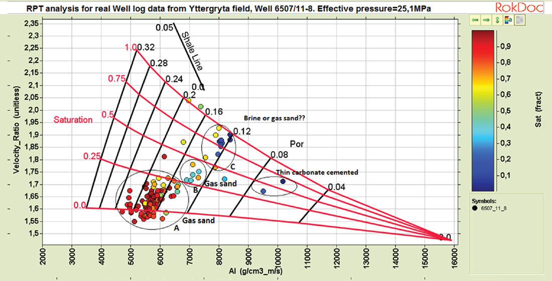
Figure 6 is a dynamic (4D) friable sand RPT for variation of pressure and saturation in the reservoir. Zone A is classified as a gas sand zone with very high gas saturation at low effective pressure. Zone B is also a gas sand zone with effective pressure between 10-25 MPa, gas saturation between 50-75% and slightly higher Vp/Vs compared to zone A. Zone C has the same effective pressure range with the lowest gas saturation between 0-35% and very high Vp/Vs.

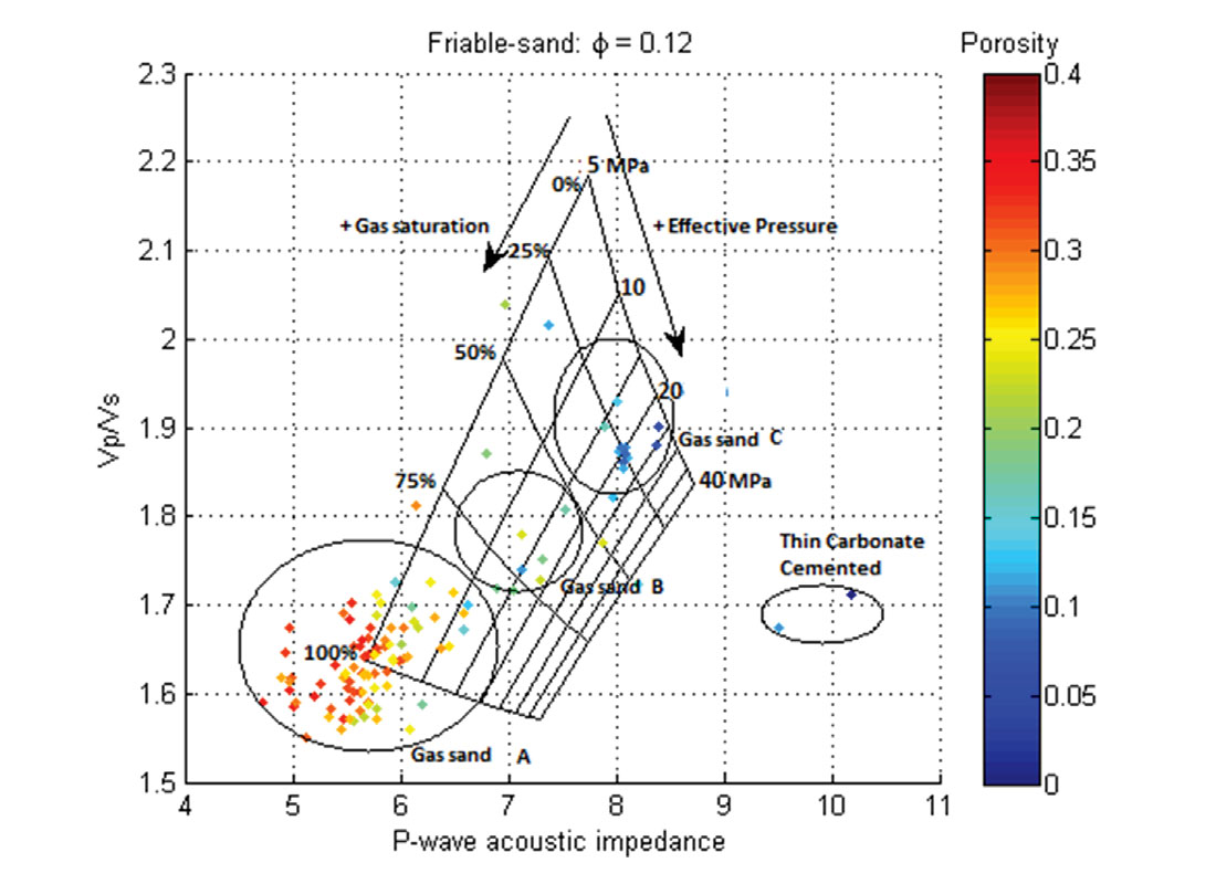
Most data points in zone A (Figure 6) are located outside the template boundaries because they have higher porosities (between 0.15-0.35) than what the RPT was constrained at.

Reservoir characterization of data using a static RPT based on patchy cemented sandstone model

The microstructure of patchy cemented sandstones can be considered as an effective medium comprising of a binary mixture of cemented sandstones, where all grains contacts are cemented, and loose, unconsolidated sands (Avseth et al., 2012).

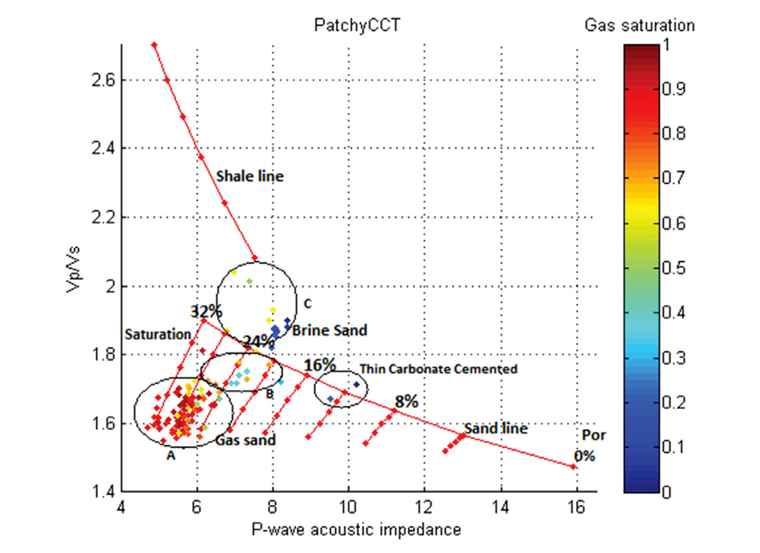
A patchy cemented sandstone model was superimposed on the Vp/Vs versus AI cross-plot domain containing data plotted for the 130 meter interval from Yttergryta field. Zones A, B, and C as defined in the previous cases were tested and predicted using a patchy cemented sandstone model, Figure 7. Plots with different color coding using gas saturation (Figure 7), porosity and shale content logs were used in the analysis and discussion. Gas saturation ranges between 0-100% in intervals of 25% and porosity from 0-32% in intervals of 4%.

Seismic Reservoir Monitoring using a Rock Physics Template (RPT)

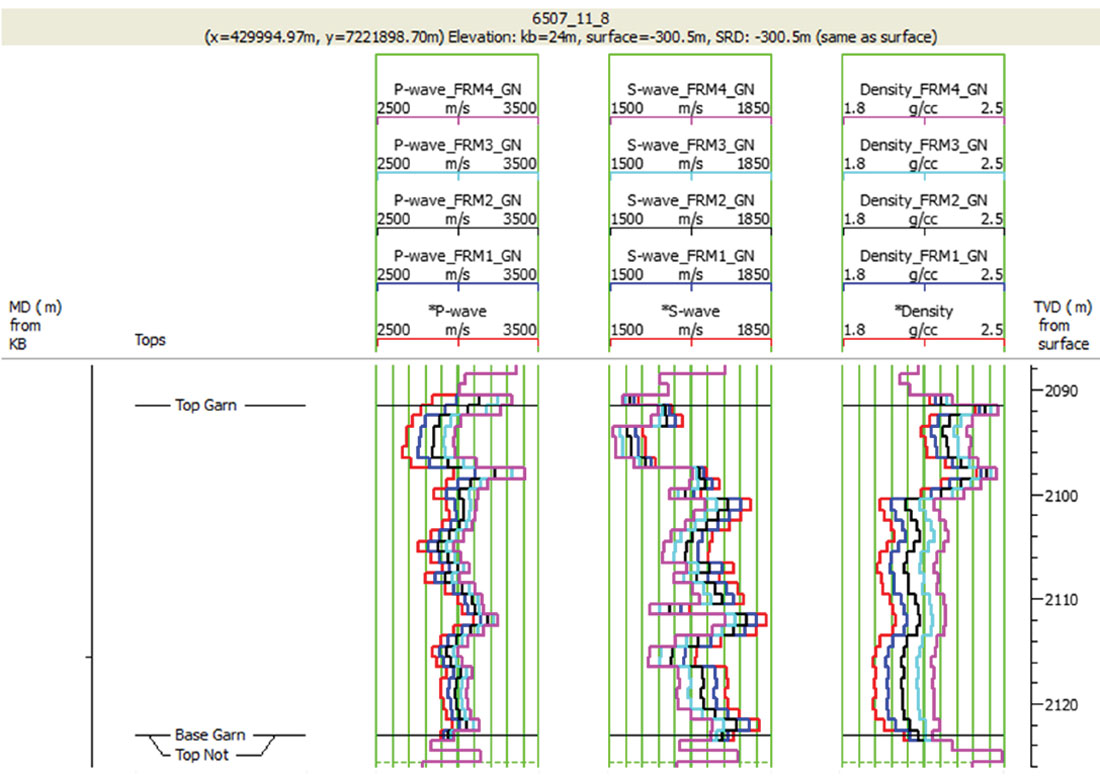
During the life of a producing reservoir the saturation of gas, oil and brine change due to either production, water/gas injection, or other activities. 4D log effects were modeled based on Gassmann’s theory; Figure 8 shows both original and fluid substituted well-log data (density, P- and S-wave velocities).

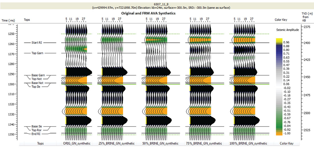
Using a zero phase, 25 Hz Ricker wavelet for angles between 5-30 degrees (near-far), AVA synthetics were computed using Zoeppritz equations for: original, 25%, 50%, 75% and 100% brine substituted well-log data. This was done to investigate how fluid saturation changes in a reservoir affect seismic data, and it is illustrated in Figure 9.

4D brine effects on seismic data in Garn Fm

To further appreciate these fluid saturation changes, the differences between the original (base) and the fluid substituted (monitor) AVA synthetics were computed as shown in Figure 10.

These encouraging results on AVA synthetics suggested that with good quality field seismic data it would be possible to see a difference in AVA responses between brine and gas filled reservoirs. After this 4D analysis on the computed prestack AVA synthetics, the results were then used in rock physics modeling (static and 4D RPT analyses). RPT analysis was then performed on both the original and fluid substituted well-log data to investigate the applicability of RPTs towards reservoir monitoring on this field. Figure 11 shows how an RPT can be used to monitor reservoir fluid saturation changes. Both original and fluid substituted log data (from Figure 8) was plotted as shown below.

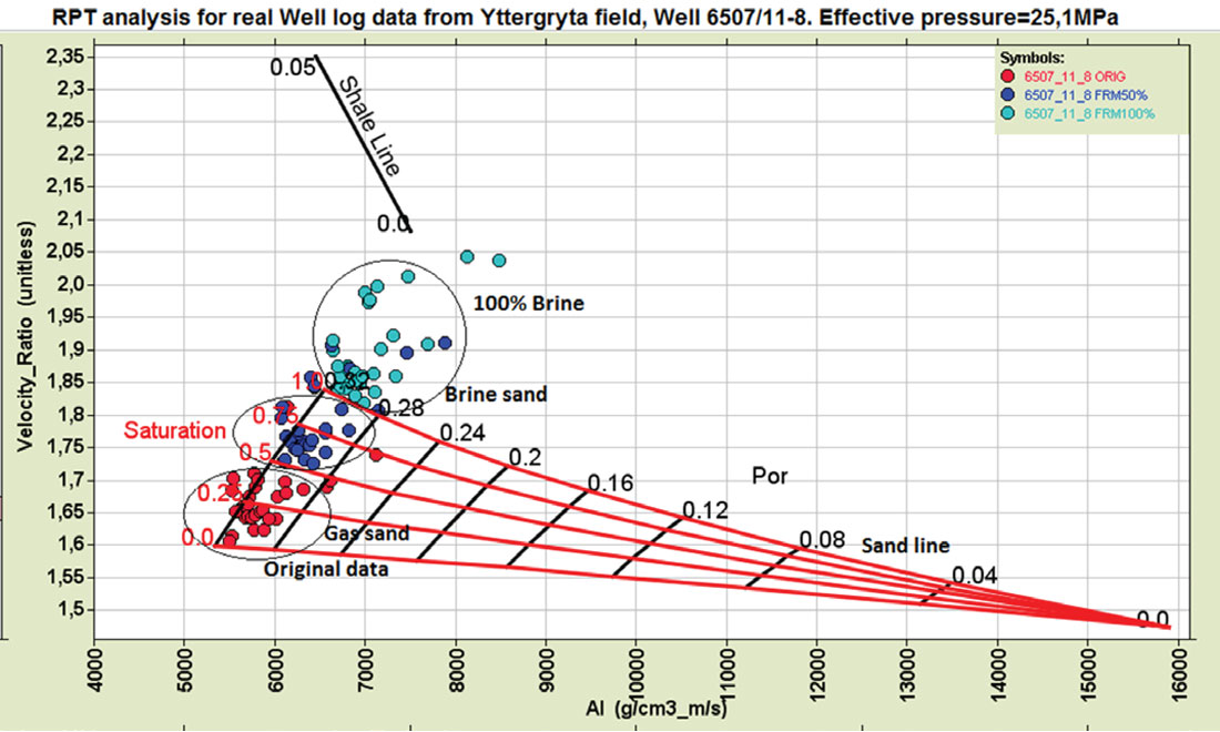
Notice the increasing AI and Vp/Vs as brine saturation increases; this causes the data points to move along the saturation lines. When brine replaces gas, the rock becomes stiffer than before and the rock bulk density increases, hence an increase in AI and Vp/Vs.

Summary

This paper detailed an integrated methodology of using rock physics templates to understand pressure, fluid and lithology effects in gas sandstones which are partly cemented. Different cross-plots of Vp/Vs versus AI with different rock physics models (contact theory, constant-cement and patchy cemented sandstone) have been discussed.

Combining P- and S-wave and density information can be very important in separation of fluid effects and lithology as it has been shown in Figure 2. Generally the sands in zone A can be regarded as tight sandstones with low Vp/Vs, (lower than 1.75). There is a small increase in Vp/Vs for sandstones with more clay (like zone B) and shales themselves have significantly higher Vp/Vs than sandstones (higher than 1.75 like in zone C).

4D rock physics templates have been used in the characterization of this data to give information on pressure variation with saturation. It has been noted that when saturation and pressure change, the data points will move accordingly. For example if pore pressure was increased this would mean a corresponding equal decrease in effective pressure. So the points would shift on the template in the direction of decreasing effective pressure. The same applies if there were changes in the fluid saturation: data points would move according to the directions indicated on the template whether increasing or decreasing gas saturation.

Conclusion

The study demonstrated how RPTs can be used in both reservoir characterization by predicting reservoir properties (porosity, lithology and fluids) and monitoring fluid changes in the life of a producing reservoir.

Acknowledgements

I thank my supervisors Prof. Tor Arne Johansen (UiB) and Dr. Erling Hugo Jensen (UiB) for the academic support, guidance and providing data. I also thank my former CSEG mentor, Matteo Niccoli of ConocoPhilips, Canada for providing helpful comments and feedback on this paper.