Rock Physics Driven Seismic Data Processing for the Athabasca Oil Sands, Northeastern Alberta

Canada has the third largest oil reserves of any country in the world. The bulk of the economically recoverable oil reserves is bitumen found in Alberta; Alberta has 26.7 Gm³ of remaining crude bitumen reserves (Alberta Oil Sands Industry Quarterly Update, Summer 2013). The Athabasca Oil Sands reservoirs of Northeastern Alberta are the primary source of this bitumen, comprising 80% of Canada’s total reserves (Wikipedia). The Early Cretaceous McMurray Formation in the Athabasca area of northeast Alberta is the main reservoir for the Athabasca Oil Sands. Based on these overwhelming statistics, it is tremendously important to understand how to process and interpret seismic data acquired from this area as robustly as possible.

Seismic data targeting the McMurray’s sandstone bitumen reservoirs should not be interpreted using the seismic stack. Rather, attributes associated with density should be used since key reservoir properties of the McMurray including porosity, saturations and lithology correlate with density but not P-impedance. Density can be extracted from wide-angle seismic data (e.g. Van Koughnet et al. 2003). Oil sands data often contain offsets sufficiently large to obtain density (e.g. Gray et al. 2006). Extraction of density implies that these data must be processed for wide angles, which is atypical of today’s industry standards. This paper examines and combines methods that we have proposed (Gray 2011, and Gray et al 2012) for improving the processing of seismic data in order to extract density information at a high enough resolution to be useful in the delineation of the reservoir properties in McMurray reservoirs. The methods described substantially improve this capability, primarily through the collaboration between processor and interpreter, to rethink the processing sequence and treat the interpretation as a problem to be solved during processing. This process results in remarkable improvements, not only in the extraction of density, but also in the imaging and resolution of this oil sands reservoir as a whole.

Basic Concepts

There are a few key concepts that make oil sands seismic data much different than conventional seismic data:

The seismic stack should not be used to interpret McMurray reservoir properties.

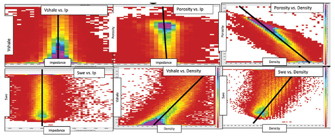
• Key McMurray reservoir properties, such as porosity, lithology or Vshale and saturation are not correlated to P-impedance (Figure 1). Therefore, attributes that are related to P-impedance, such as the stack, intercept, or P-impedance inversions, should not be used to interpret McMurray reservoirs.

The McMurray reservoir should be interpreted using density.

• Key McMurray reservoir properties, such as porosity, lithology or Vshale and saturation are correlated to density (Figure 1). Therefore, attributes that are related to density, such as density reflectivity, density inversion and ultra-far angle stacks, should be used to interpret McMurray reservoirs.

Oil sands seismic data should be processed using azimuthal velocities.

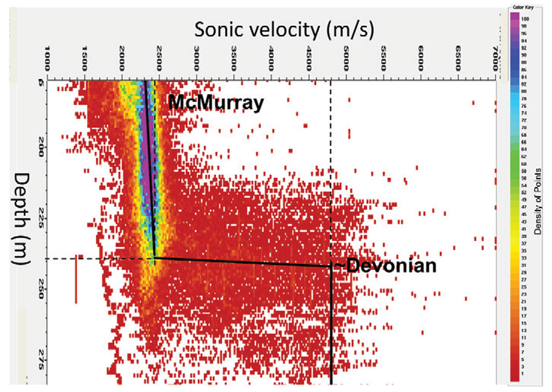
The Early Cretaceous McMurray Formation – Devonian unconformity interface is a sizeable 100% (2400 m/s to 4800 m/s) velocity contrast (Figure 6).

• The McMurray reservoir is shallow with a variable depth ranging over 160m – 260m in this area.
• The McMurray reservoir is very attenuative.

The seismic stack should not be used to interpret McMurray reservoirs

Figure 1 shows that from hundreds of wells there is no consistent correlation between P-impedance and any of the key parameters that we use to distinguish McMurray reservoir properties including: porosity, saturations, lithology, facies, net-to-gross or weight of tar. In all the McMurray reservoirs the authors have seen, this lack of correlation of reservoir properties to P-impedance and the stack has always been the case. Geophysicists struggle to interpret these reservoir properties between wells using conventional techniques. It is thus our conclusion that any seismic attributes related to P-impedance should not be used to interpret the McMurray reservoir properties. Since the seismic stack is generally considered to be a representation of P-impedance changes, the stack should not be used to interpret McMurray reservoir properties.

The stack is not without value. A properly processed P-wave stack provides the interpreter insight into the general structural and depositional regime of the area. Use the stack to understand and interpret the Devonian and caprock, but do not rely on the stack exclusively to interpret the McMurray reservoir.

Density should be used to interpret McMurray reservoirs

We have consistently observed significant correlations between density and the key parameters that we use to distinguish McMurray reservoir properties such as: porosity (~80%), saturations (~60%), lithology (~70%), facies (~70%), Vshale (~70%) and weight of tar (~65%). Figure 1 shows examples of such correlations from a dataset consisting of 600 wells across more than 100 km2 of McMurray reservoir. Density can be derived from oil sands seismic data (e.g. Gray et al, 2006), and it can be used to assist in the interpretation of McMurray reservoirs (e.g. Archer et al, 2013).

Long offsets must be kept during the processing of oil sands seismic data, since the bulk of the information about the density is considered to be in wide angles. The shallow McMurray reservoir works to our advantage because wide angles and long offsets are commonly acquired at this depth. In order to properly resolve refraction statics for this shallow reservoir at about 150-250 m, offsets of several hundred metres are required. With shallow McMurray reservoir depths, we frequently have sufficiently long offsets to get to the far (~1.5X) and ultra-far (>2X) offset-to-depth ratios required to estimate density.

The properties of the McMurray reservoir come to our rescue in another way, which is not as well known or understood. McMurray sands are considered to be unconsolidated and under-pressured. This means that the McMurray elastic behaviour approximates that of slurries. Slurries act as liquids because they have no shear modulus, so if there is an AVO effect in a slurry, then what causes it? Since there is no shear modulus in a slurry, then density is the only parameter that can change the AVO behaviour in it. Therefore, it is probable that AVO responses in the McMurray might have more to do with density than with shear properties. Figure 2 (after Gray 2003) seems to support this. The density reflectivity extracted from 3-term AVO inversion seems to correlate with the well log density synthetics far better than the S-impedance reflectivity does with shear impedance synthetics.

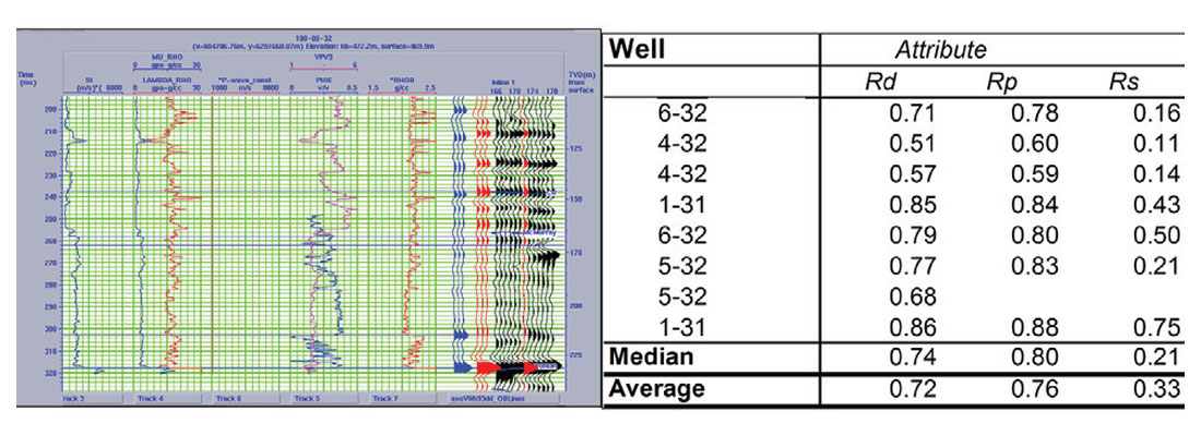
The very wide angles (>45°) are often available in shallow data because long offsets (relative to the shallow depths of these targets) are required to solve the near-surface statics solution. For example, in these data, there are 900 m offsets available and the base of the reservoir is ~250m. These long offsets provide angles of more than 60° in the reservoir and above. The possibility to extract density while limited to data that have only conventional angles may also exist, due to the similarity of the McMurray reservoir to a slurry. Density is correlated to the key reservoir properties and P-impedance is not correlated to any key reservoir properties (Figure 1). Note that the Rp section is correlated to the P-impedance well log in Figure 2, but the P-impedance well log is not related to any key reservoir properties, as shown in Figure 1. Therefore, the Rp section is not correlated to any key reservoir properties. Therefore, density should be used to interpret McMurray reservoir internal architecture. At a minimum, a far (≥30°), or preferably an ultra-far (≥45°), stack should be used to interpret the McMurray since the far offsets contain density information that ties to these key reservoir properties.

Oil sands seismic data should be processed using azimuthal velocities

There are many considerations for keeping long offset data in the processing sequence; the most important being anisotropy. Surprisingly, for these shallow, unconsolidated sands, resolving azimuthal (HTI – horizontal transverse isotropy) anisotropy, not polar (VTI – vertical transverse isotropy) anisotropy is the key. There are significant azimuthal variations in moveout that start to appear at wide angles. The cause of these variations is not presently understood. What is important is that these variations exist. To get reliable estimates of isotropic density from these wide angles, the effects of azimuthal velocity variation must be removed. Figure 3 shows that, for conventional AVO angles within 30 degrees, azimuthal variations do not seem to matter.

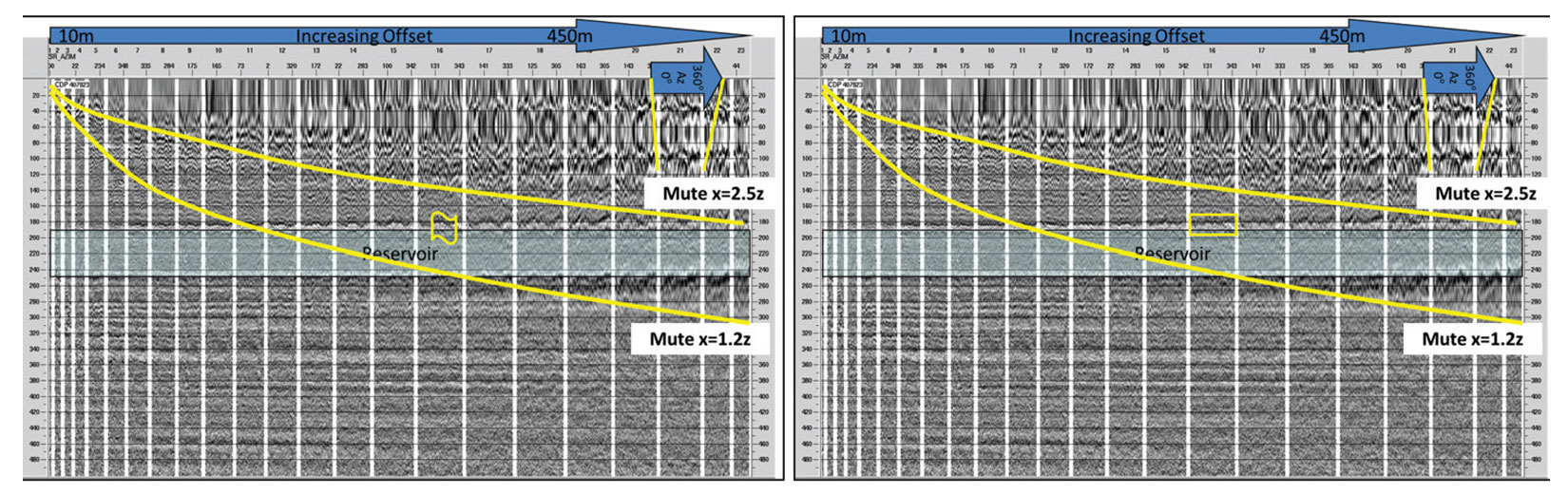
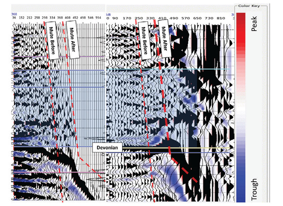
Past 30 degrees, the azimuthal variations seen in the COCA (Common- Offset, Common Azimuth) cubes (Gray, 2007) in Figure 3 will cause destructive interference damaging the far and ultra-far angles. Minimal background anisotropy of about 3% is all that is required for this interference to happen. This is about the level of background anisotropy in the earth (Crampin, 1998). Velocities in the near-surface are very slow. A weathering velocity of ~600 m/s, and a replacement velocity of 1800 m/s is used in the processing. These processing velocities are determined from data and knowledge of the area. They are representative of the velocities to be expected in the shallow section. Such slow velocities result in the seismic wave spending more time in the shallow section. Even minor anisotropy effects are exacerbated here and, for velocities, these effects will be observed down to, and past, the reservoir level unless an orthogonal anisotropy is encountered. At a depth of 200 ms in another oil sands dataset we have processed, we have seen 20 ms of azimuthal moveout at angles of about 60 degrees. In order for that amount of moveout to happen an average anisotropy above only 6% is required because of the slow velocities in the near surface. In our dataset, 10 ms of azimuthal moveout at 200 ms and 320 m offset can be seen (Figure 3). The dominant wavelength of these data is about 5-6 ms. This azimuthal moveout, if uncorrected, will cause stacks of all these azimuths to destructively interfere, destroying the AVO effect, as shown on the left side of Figure 4. If azimuthal moveout is incorporated, an additional 25% more offsets can be included. These are the offsets that contain the bulk of the information required to determine density.

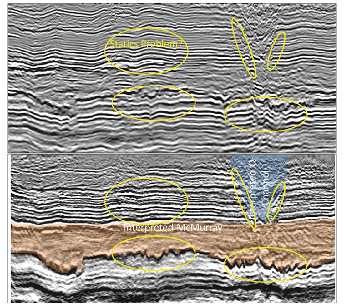
Improvement of the stack is an additional benefit derived from correcting for the higher order move-out attributed to azimuthal anisotropy. In the example shown in Figure 5, imaging of the entire section, from quaternary to Devonian, has improved substantially by incorporating azimuthal velocities in addition to other methods recommended in this paper. The imaging of the Devonian has improved substantially, indicating fine-scale karsts at the top of this carbonate unconformity. The edges of a shallow Quaternary channel, incising into the Cretaceous are now imaged with the new methods. IHS (inclined heterolithic strata) beds of the McMurray reservoir are also imaged more clearly in some areas with azimuthal velocities.

Improving the wider angle data through the use of azimuthal velocities has resulted in significant improvements in the seismic data, which help to better image the reservoir and the formations around it.

The McMurray – Devonian interface is a sizeable velocity contrast

Figure 6 shows that the velocities jump from ~2400 m/s at the base of the McMurray to ~4800 m/s in the carbonates of the Devonian (Gray et al, 2012). The McMurray-Devonian contrast is so large that the seismic data can effectively be considered a half-space. As a result, all other reflections, including those from the reservoir, are effectively noise to some of the processing algorithms and careful attention must be Figure 5. The seismic stack with isotropic velocities (top) and anisotroic velocities (bottom). Ellipses highlight areas where significant improvements have occurred. The lowermost changes are on the Devonian reflector, which is at the bottom of the brown Interpreted McMurray section. The ellipses on the upper right highlight channel edge reflectors that can occasionally be seen in the new processing. The ellipse on the upper left highlights a more accurate depiction of caprock structure after improving residual statics procedures. paid to the data around the McMurray – Devonian interface. There are some important processing considerations that emerge from this sizeable velocity contrast

1. Shear-wave velocities in the Devonian are similar to P-wave velocities in the McMurray.

2. The McMurray-Devonian interface dominates all cross-correlations,

eg.

1. Statics
2. Deconvolution

Shear-wave velocities in the Devonian

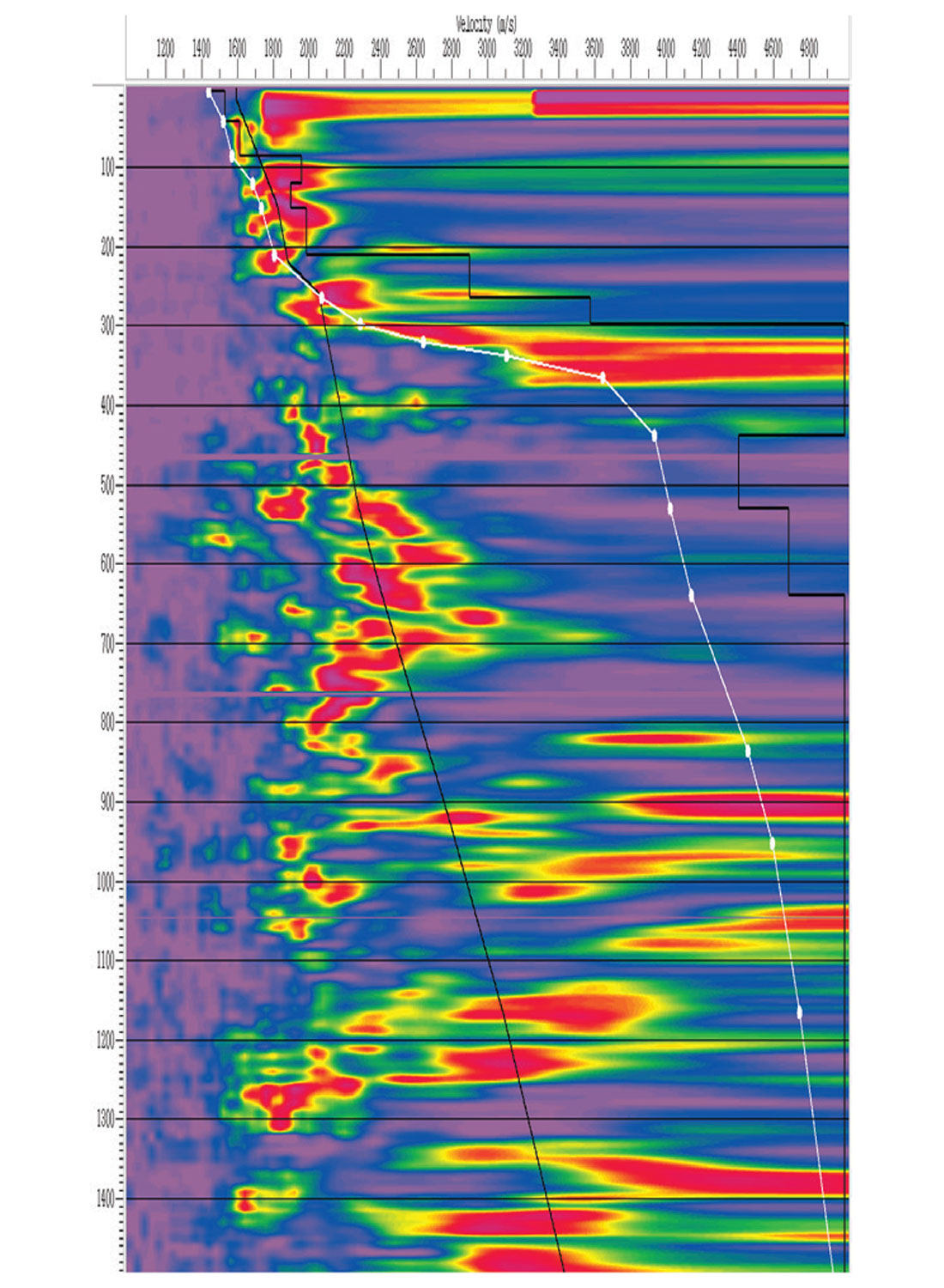
The shear-wave velocities in the Devonian are on trend with the P-wave velocities in the McMurray. The Devonian P-wave velocities are about twice the P-wave velocities in the McMurray, but the Vp/Vs ratio in carbonates is about 2 (Pickett, 1963). Therefore the S-wave velocities in the Devonian carbonates are about the same as the P-wave velocities in the McMurray. Seismic data processors are trained to follow a velocity trend. Therefore, without additional information, a well-trained processor will follow the shear-wave velocities in the Devonian section in these data. Following this trend can result in erroneous velocity picks in the Devonian. This is where an interpreter helps by providing guidance to the processor, regarding where the velocities trend should be based on well logs. An example of this guidance is shown in Figure 7, where the correct stacking velocities follow the white line, producing interval velocities (jagged black line on the right) of about 5000 m/s at the top of the Devonian at 300 ms in the Figure. The smooth black line on the left follows a trend of what appear to be PSSP reflections. This velocity trend produces a slight increase in interval velocity at the top of the Devonian, but this increase was not close to that observed in the well velocities. The velocities were corrected, and the white velocity trend was used in this processing sequence. These faster velocities, informed by the interpreter, significantly improve the interpretability of the data in the deep section below the Devonian unconformity (e.g. Figure 8).

The McMurray-Devonian interface dominates all cross-correlations

The large velocity and density contrast at the McMurray – Devonian boundary is so strong that it dominates all other reflections in the section, effectively making this section like a half-space. Some important processing algorithms use correlation techniques, including deconvolution and statics. The correlation function effectively squares the amplitude of the traces, so that the substantial McMurray – Devonian reflection dominates these algorithms. The implications of the correlation are important, especially because the McMurray is very attenuative and the Devonian surface is rugose in this area. An attenuative McMurray means that the seismic wavelet has lost much of its high frequencies by the time it gets to the Devonian. Since the McMurray – Devonian interface dominates the autocorrelation that drives the deconvolution, the deconvolution is done on a more limited frequency range than it should be. The rugose Devonian, in combination with the domination of the cross-correlation by the McMurray – Devonian boundary, means that, if they are not handled properly, structures can be induced by a residual statics algorithm.

Deconvolution

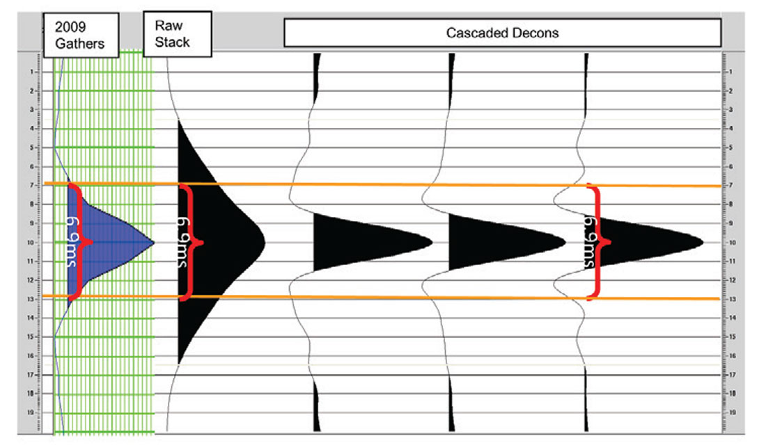
The thickness of layers that are considered barriers to fluid flow in the McMurray vary from project to project, ranging from 1 – 3 m, with an average of 2 m. We can use this range to determine the seismic data frequency content that would be required to resolve a 2 m barrier. Using the λ/4 rule (Widess, 1973), the wavelength (λ) required to detect a 2 m barrier is at most 8 m long. In this project the sonic velocities in the McMurray average 2350 m/s (Figure 6). This velocity means that a wavelength of at most 6.9 ms, or a dominant frequency of 146 Hz, is required to see these barriers. Fortunately, these frequencies are available in these data (Figure 9).

The original deconvolution (decon) does not produce a wavelet short enough to image these barriers in the stack, though there is enough frequency content to use tools like spectral decomposition. The attenuation in the McMurray and the dominance of the McMurray – Devonian boundary in the cross-correlation may have also affected the wavelength. We decided to use a different strategy to boost the frequency content and thereby shorten the wavelength. A useful rule of thumb used in deconvolution and wavelet extraction is that there should be 4-6 wavelets, or operators, in the window used to deconvolve or extract the wavelet. The idea behind this is that there needs to be enough wavelets to average out the background earth reflectivity. For example, if the wavelet was as long as the window, the deconvolution process (without pre-whitening or other constraints) produces a reflectivity series of single spike with a wavelet shaped like the reflectivity sequence in the window. Therefore, more than one wavelength is required for the window length. The bandwidth of the data provides information on the length of the wavelet. The minimum length of the wavelet has to be more than the inverse of its minimum required or expected frequency, f, to be recovered by the fundamental relationship λ = 1/f. Using this logic, and the roughly 200-300 ms window of seismic data down to the base of the McMurray in our dataset, we could only use a deconvolution operator of a maximum of 60 ms. A 60 ms operator can only see down to a minimum frequency of the inverse of its wavelength, 1/λ (in this case 17 Hz because its wavelength is its maximum period). Realistically, more than one period is required for deconvolution to properly recover a given frequency band. In our experience, an operator of 60 ms can only realistically deconvolve down to a frequency, f =2/λ, because there is not enough information to properly recover the wavelet in a single wavelet for the reason stated above. The 60 ms wavelet can therefore only see >34 Hz. This high minimum frequency is a problem because ultimately, we want to invert for density. These lower frequencies need to be filled in. The solution in this dataset comes by cascading deconvolution operators. The first deconvolution uses a long operator and a long window, in our case 160 ms and 800 ms respectively. The longer window respects the rule of thumb above. The longer window allows us to get down to frequencies of ~10 Hz. The longer window does not deconvolve the higher frequencies that we determined were needed to see shale barriers. Deconvolution of the higher frequencies is done by a second deconvolution, where we use the 60 ms wavelet over 300 ms to get the high frequencies. Both deconvolutions require much higher pre-whitening, because the pre-whitenings are effectively squared by the cascading processes (e.g. two cascaded operators with 10% pre-whitening effectively become 1% when combined).

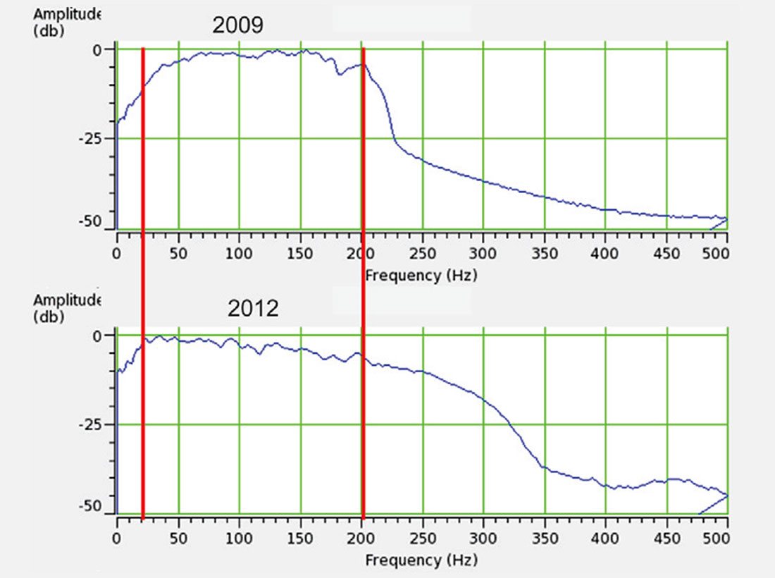
Wavelet phase is most sensitive to the low frequency component of the amplitude spectrum. Efforts were made to minimise noise, prior to deconvolution, via modeled shot-derived noise attenuation and the judicious use of trace edits. The first stage of the deconvolution flow used a minimum phase operator, designed to include a low end frequency of 6.25 Hz (in a 160 ms operator). With the assumption that that phase was stabilised in the low frequencies after minimum phase deconvolution, the spectra of the data was broadened by cascading the data into a shorter zero phase operator. Data below 17 Hz (corresponding to a 60 ms operator) were not affected by the zero phase deconvolution. This methodology satisfies the need for both high and low frequencies (Figure 10). An extra half octave at the high end and an extra octave at the low end are achieved. The extension of the frequency band creates a dominant frequency that meets our needs (Figure 9).

Statics

There are two forms of statics: refraction and reflection statics. The latter are usually referred to as residual statics. Refraction statics provide guidance as to where the reflectors should lie. There can be a problem with residual (reflection) statics if the strong McMurray – Devonian reflection is not taken into account. Residual statics help to improve these seismic data, but early attempts created artificial structures in the caprock (e.g. the upper left ellipse in Figure 5). Most statics procedures assume that the raypath in the near-surface is near-vertical because of the very low velocities expected there. If that assumption is true, then statics can be iteratively applied as a single value to each individual pre-stack trace. E.g refraction statics might shift the trace by +20 ms, then the residual statics might shift that same trace by -2.5 ms, for a summed total shift of that single trace of 17.5 ms. Other traces will each have their own single value. If there are high velocities in the near-surface, then statics are more properly corrected with migration techniques. If time-variant statics seem to be required, we would recommend looking at azimuthal velocities and then applying a single static. One form that the process of residual statics takes is creating a model, then moving individual pre-stack traces up or down to match that model by using a bulk-shift determined from cross-correlation of that trace to the model. The model is generally a highly noise-attenuated and smoothed version of the stack. The process of smoothing a rugose reflector, in combination with the strength and rugosity of the McMurray – Devonian reflector causes the problem. The model smooths through rugose structures, making them smoother and therefore flatter. The result of this smoothing can be seen in the McMurray – Devonian reflector in the lower-left ellipse in the upper stack in Figure 5. Other reflectors that are not as strong, such as the caprock reflectors in the upper-left ellipse in Figure 5 are also affected because only one static value is applied to each trace. When there is a strong, rugose reflector with structure different than the surrounding formations, it is generally worthwhile to not move too far from the refraction statics solution. If the McMurray – Devonian reflector amplitude is knocked down sufficiently so that it does not drive the cross-correlation, residual statics can be done. We are able to get a good residual statics solution in these data by knocking down the McMurray – Devonian reflector amplitude with an offline 50 ms AGC (automatic gain control) process, which effectively equalizes the amplitudes over a running 50 ms window. The 50 ms AGC is applied to both the individual traces and the model. The AGC knocks the McMurray – Devonian amplitudes down to the same level as surrounding reflectors, so that they no longer dominate the cross-correlation. As seen on the bottom of Figure 5, the results show a more reasonable structure, consistent with the refraction statics solution, which does not appear to introduce artificial structures in the caprock. Artificial structures, like those seen in the upper section in Figure 5, are caused by the single static and incorrect smoothing of the residual statics model. These artificial structures could cause an erroneous interpretation of higher caprock stress. A more consistent structure allows for a more appropriate interpretation of the caprock stress in this area.

Discussion

By revisiting processing, in the context of the very specific requirements for oil sands data, it has been discovered that significant improvements can be made on data that are already quite good. The important thing is to think through the processing sequence as a problem-solving exercise. Many of the improvements made to these data came about by rethinking how to use common processes on these data. Improvement comes naturally when you ask the question: “What should I do to most efficiently and effectively provide the information that my colleagues need from these data?” Work with the geophysicists, geologists and engineers on your team, and include the seismic data processors, to get to that answer. These results could not have been produced without the combined efforts and discussions of both interpreters and processors thinking about an engineering-focused final objective.

Value

There is much value to be gained by optimally utilizing all the collective tools we have. This exercise is an example of extracting more value through the intelligent use of existing tools on data that most geophysicists would consider to be extremely good. This is best done with an objective in mind. In our case, the objective is to extract the best possible density information from the data. Petrophysical analysis shows that density is the key to extracting value from these seismic data because density is the one elastic parameter that correlates with the reservoir properties of interest: saturation, porosity and lithology. The extraction of density cannot be done well with the seismic gathers that produced the good quality stack that we had because these gathers did not have the necessary angle coverage to stably extract density. Therefore, reprocessing for wider angle coverage is necessary. The objective, in this case wide angles for density, determines which processing tools are required. In our case, the tools included using anisotropic velocities to stabilize the offsets. Along the way, we discovered that the statics and deconvolution could be improved. The new deconvolution improves the bandwidth by an octave at the low end, which is very important for the density inversion, because it means that more seismic data and less interpolated well information is used in the inversion. This density inversion is used to predict porosity, lithology, saturation and caprock strength, which are parameters that reflect the value of this reservoir.

Conclusions

We have improved the usefulness of what was formerly well processed seismic data. In particular, we have determined that the best attribute to derive from oil sands seismic data is density, because it correlates with key reservoir properties that impact the assessment of the reservoir, e.g. porosity, saturation and Vshale. The correlation of density with key reservoir properties was demonstrated using cross-plots of hundreds of wells across the McMurray. Density can be derived from wide-angle seismic data that is often available in shallow oil sands plays. Conversely, the seismic stack is inappropriate to determine reservoir properties because it shows no consistent correlation with reservoir properties, at least in any of the many reservoirs that we have seen. The stack is not useless. It can, and should, be used for the interpretation of the Devonian and the caprock. The notion that density is important for McMurray interpretation led us down a path where we discovered that we needed to rethink certain elements of the processing sequence in order to optimize the interpretation. In particular:

• Azimuthal velocities improved the far offsets by removing destructive interference, resulting in 25% more of the longest offsets required to stabilize the density estimates.
• By checking that processing interval velocities are similar to well log velocities in the Devonian, a risk of misinterpreting shear reflections as PP reflections has been eliminated.
• By examining and improving the deconvolution process, both high and low frequency content has been significantly enhanced. In our example, by ½ octave from 200 to 300 Hz on the high end, and by a full octave from 40 to 20 Hz on the low end. Higher frequencies mean shorter wavelets, which improve the ability to see barriers in the McMurray. Lower frequencies mean that fewer frequencies need to be filled in from well control, etc. when doing inversion.
• By examining the statics process, inconsistent structures in the caprock have been removed. This results in seismic data that are more consistent structurally and therefore are more appropriate for analyzing caprock.

The combination of all these techniques has produced seismic sections that are more representative of the geology and reservoir properties that we need to interpret. These seismic sections are more useful for creating volumes to pass on to our colleagues for reservoir characterization and simulation.

Simple problem solving has resulted in a substantially improved seismic section that is more appropriate for the interpretation and reservoir characterization that geophysicists need to do in oil sands projects today.

Acknowledgements

We would like to thank the following people and organizations for the contributions that they have made to this article: Lee Hunt, Amanda Knowles, Ashley Gray, Penny Colton, Sissy Thiesen, Dragana Todorovic-Marinic, Elizabeth Earl, Ed Jenner, Richard Bale, Doug Horton, Kim Head, Bob Batt, Nader Gerges, Bruce Palmiere, Edwige Zanella, Jaclyn Chernys, Randy Cormier, Corrina Bryson, Wayne Hanson, Wes Siemens, Paul Anderson, Jay Gunderson, Kristof DeMeersman, Ken Tubman, Carmen Dumitrescu, Rick Ogloff, Eric Andersen, Barry Wright, Scott Haffner, Scott Cheadle, Edwige Zanella, Tricia Chrzanowski Nexen Energy ULC, Ion Geophysical Corporation and CGG Canada Services Ltd.