Revisiting the Radial Trace Transform

Introduction

In geophysics, as with many other disciplines, it can sometimes be fruitful to review an idea originally conceived many years ago for one particular application, to see whether it can also be used for other purposes. The radial trace transform is an example of such an idea. Originally introduced by the Stanford Exploration Project (Claerbout, 1983) mainly to assist in migration and imaging, the radial trace (R-T) transform has subsequently found other uses because of its unique geometric distortion of the wavefield. One of the better known applications, long-period multiple attenuation, was introduced by Taner (1980) and subsequently refined by Lamont et al (1999). The purpose of this article is to introduce the reader to more uses for the R-T transform. One of these, coherent noise attenuation, has proven to be especially effective, in some cases achieving better noise suppression than more traditional F-K or Tau-P transform techniques, while preserving lateral wavefield detail such as event terminations and static shifts.

Radial trace transform defined

Many geophysicists confuse the radial trace transform with the Tau-P transform, because the two were introduced to seismic processing at about the same time for much the same purpose. While the two transforms have similar co-ordinates, the better known Tau-P transform is an integral transform, while the less prominent radial trace transform is a simple point-to-point mapping. The R-T transform extracts wavefield amplitudes from a seismic trace panel, such as a shot or receiver gather, and interpolates them onto coordinates of velocity and travel time. Figures 1 and 2 illustrate the mechanics of the mapping operation.

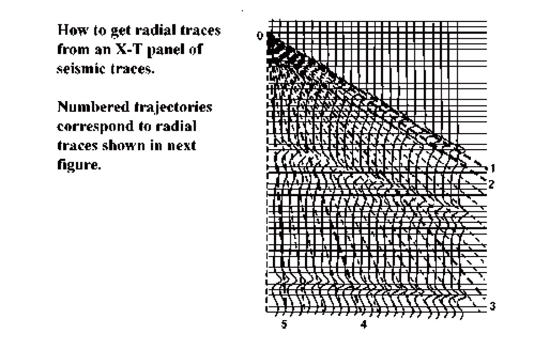
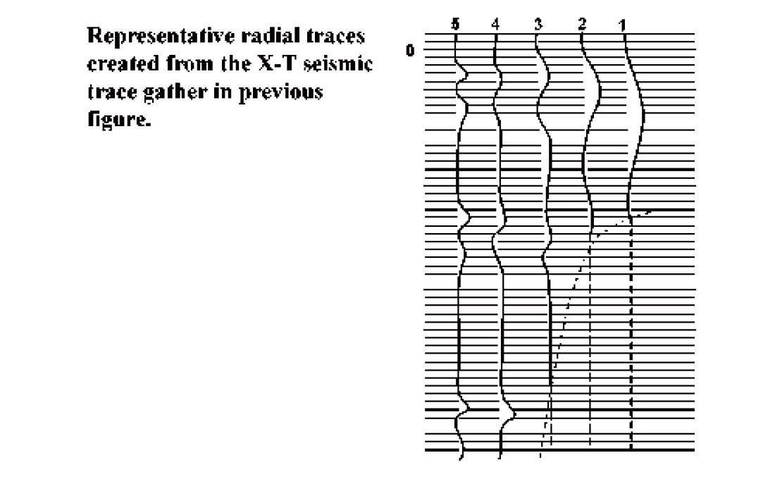
Figure 1 shows a schematic shot gather with co-ordinates of offset distance (X), and travel time (T). Overlaid on this gather is a fan of common-origin radial trace trajectories, each having a unique velocity. To map seismic amplitudes from the shot gather to the radial trace domain, all the amplitudes intercepted by a particular trajectory are transferred in sequence to the new domain as a single radial trace; and the process is repeated for each trajectory. Figure 2 contains a few representative radial traces corresponding to the numbered trajectories in Figure 1. It is important to note that by definition the radial traces and X-T traces share the same time scale and sample interval. This means that samples required by a radial trace often fall between the discrete X-T trace samples and must be interpolated from nearby values. Because there are many possible interpolation methods, this part of the R-T transform algorithm can be tailored to suit the desired application. While for many purposes, interpolation along the X-direction is appropriate, interpolation along radial trace trajectories can also be done and may be more appropriate in some cases (Brown and Claerbout, 2000). Likewise, interpolation methods can be chosen which use only nearest neighbour values for interpolation, or which involve other nearby points as well.

A useful distortion

One of the peculiarities of the R-T transform that makes it especially useful for coherent noise attenuation and wavefield separation is illustrated in Figure 2: the stretching of the waveform of any linear event intersecting the R-T transform origin. Because amplitude values gathered along a radial trace trajectory almost parallel to a linear wavefront come from nearly the same point on the waveform on each X-T trace, the resultant radial trace only varies slowly with time. Thus a coherent linear event whose X-T domain frequency spectrum lies in the normal seismic band appears to contain mainly sub-seismic frequencies in the R-T domain. Events like reflections, that do not pass through the R-T origin undergo little distortion, however, since the radial trace trajectories cross the wavefront at a steep angle, thereby capturing the high frequency variation. This mapping of common-origin linear events into very low frequency radial traces is what enables coherent noise attenuation and wavefield separation. Applying a low-cut filter to the radial traces attenuates the energy mapped from linear events which intersect the radial trace origin while passing the energy of events, like reflections, which don’t. Alternatively, applying a low-pass filter in the R-T domain attenuates reflections and passes linear, common – origin events.

To further understand the radial trace perspective with respect to a linear wavefield event, consider paddling a surfboard straight out into the surf, directly into the face of a wave. The surfer rises and falls rapidly as he crosses a wave perpendicular to the wavefront: the X-T trace perspective. When the surfer “catches a wave”, however, he moves nearly parallel to the wavefront, and travels the length of the wave, neither rising nor falling very much as he moves along the wavefront: the R-T point of view. X-T traces sample across linear wavefronts while radial traces sample along them.

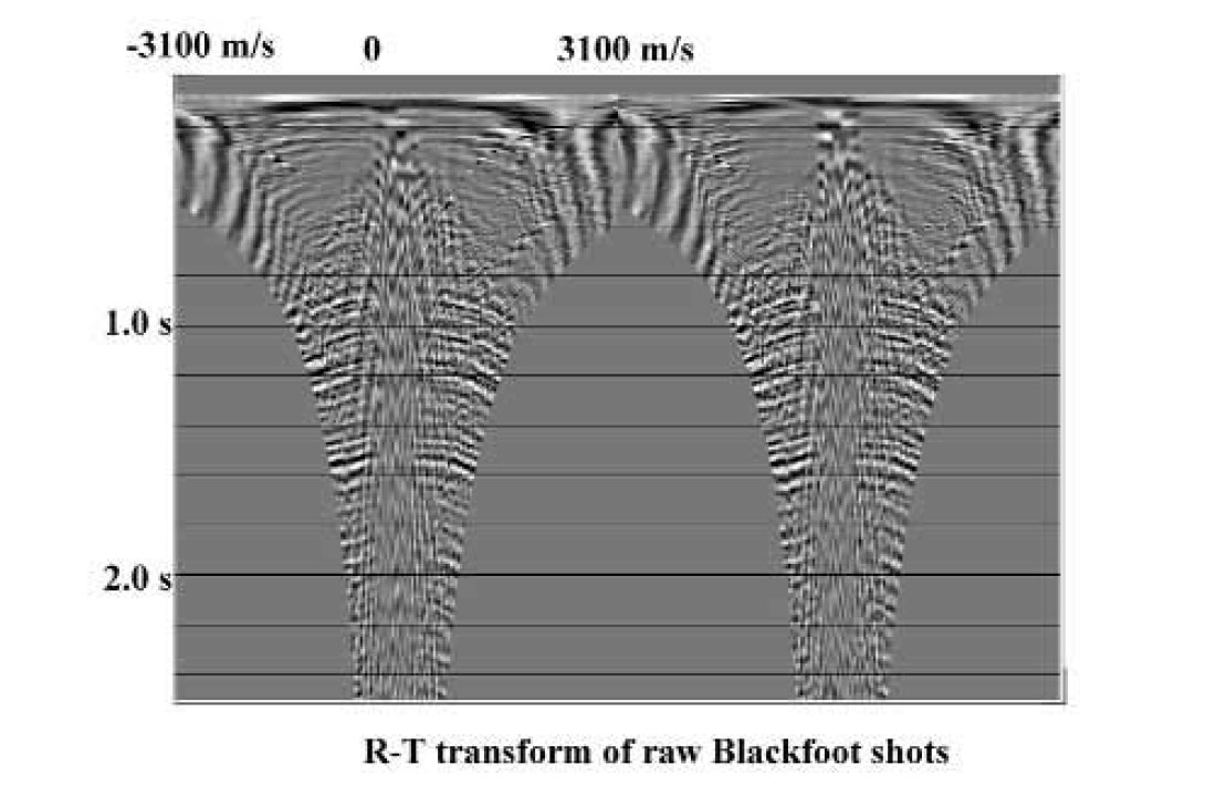
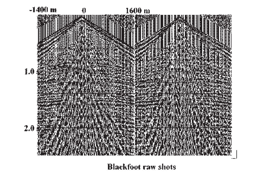
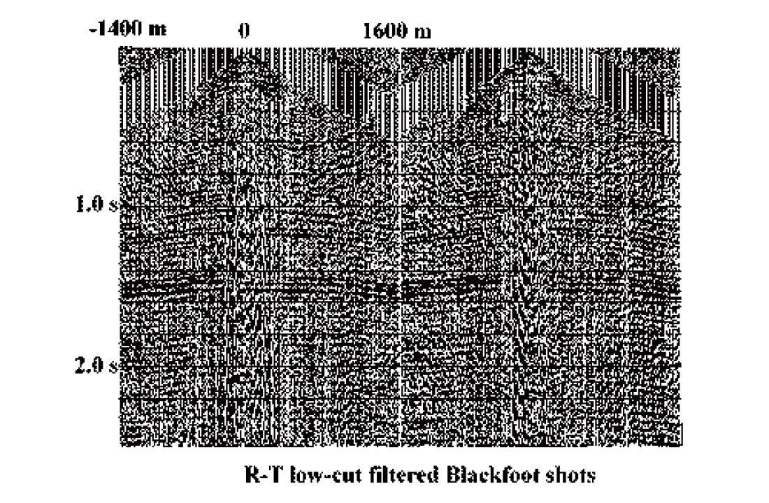
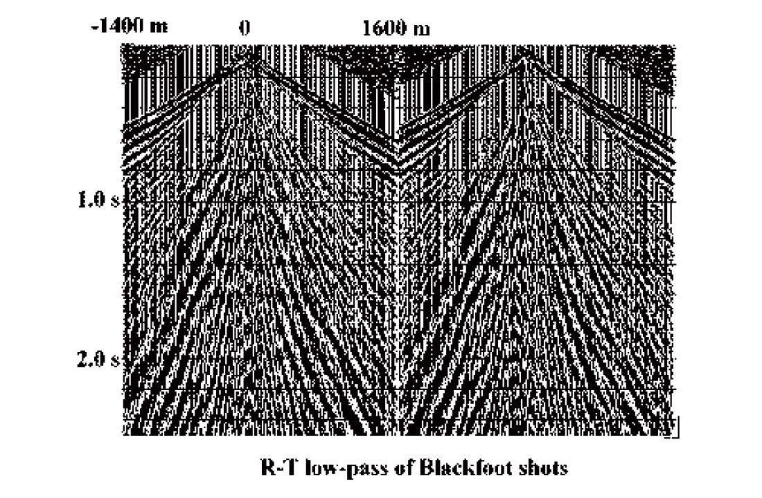
As a demonstration of the R-T transform and its distortion of XT space on real data, Figure 3 shows two shot gathers containing several types of coherent noise, from a seismic survey at the PanCanadian Blackfoot field. Figure 4 displays the R-T transforms of the shot gathers, where care has been taken to place the transform origins at the apparent common source points of the coherent noise modes on the shot gathers. The low-frequency events mapped to the high velocity edges of the radial trace gathers are the direct arrivals and related modes, while those in the low velocity centre of the gathers are the ground roll and air blast. Application of a low-cut filter in the radial domain, followed by the inverse transform to X-T, results in the considerably cleaner shot gathers of Figure 5, while a low-pass filter and inverse transform applied to the radial traces yields the coherent noise shown in Figure 6.

Coherent noise attenuation

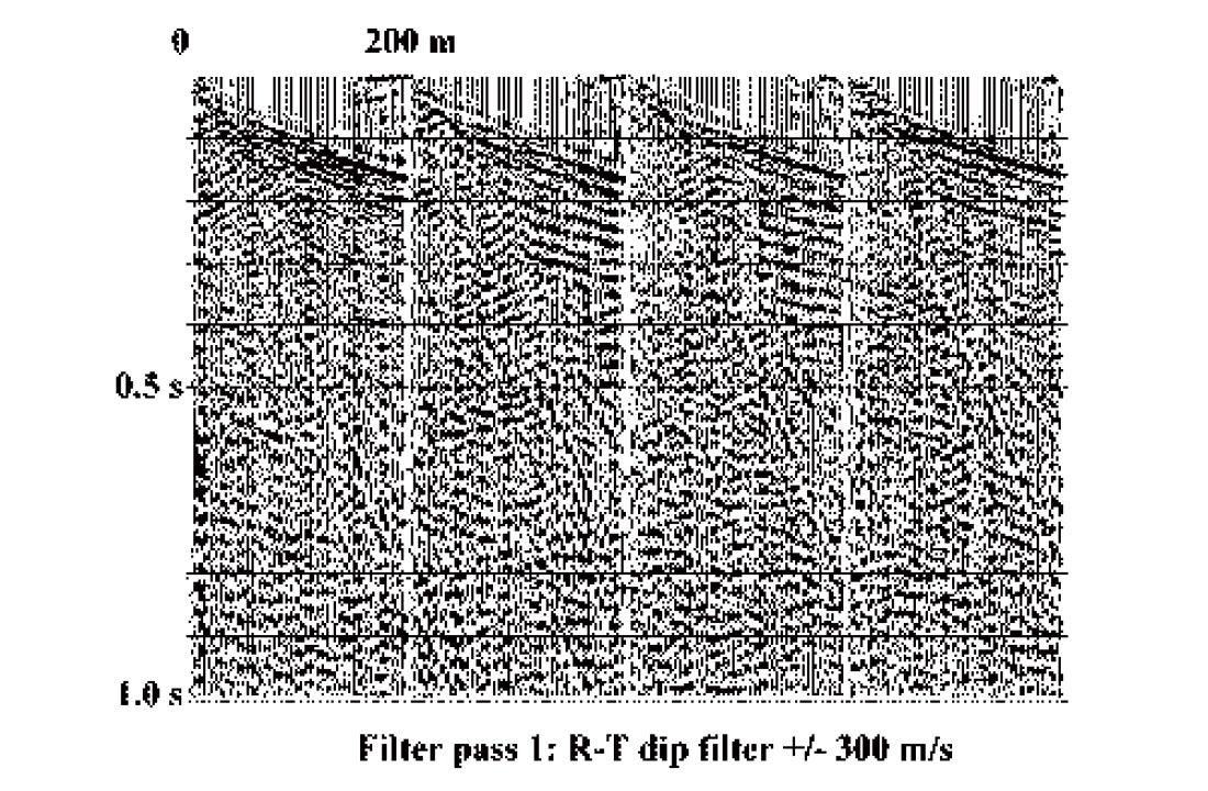
One of the main advantages of the R-T transform with respect to other transforms is the ease with which it can be tailored to fit a particular manifestation of coherent noise. In addition, R-T filter passes can be cascaded, so that individual noise components can be attacked using specifically designed filters. The freedom to place an R-T transform origin anywhere in virtual space means that in addition to the radial ‘fan’ filter process illustrated above on the Blackfoot data we can also implement a ‘dip’ filter process. The RT ‘dip’ transform is simply a thin ‘fan’ transform with a narrow range of radial trace velocities (or ‘dips’) and a distant origin, located so that the target gather is fully covered by the R-T fan. An appropriate filter applied to radial ‘dip’ traces then attenuates (or emphasizes) linear X-T events aligned with the radial traces. As an example of this application, Figure 7 shows raw shot gathers from the 1998 Shaganappi geotechnical survey done on the University of Calgary reserve lands. The use of a surface source here has resulted in a very high level of source-generated noise, and the relatively low fold of the survey means that the noise must be attenuated before stack. If unabated, the noise on the shot gathers results in the unsatisfactory stack image of Figure 8. In this figure, there are a few apparent shallow events, but some of these are actually fortuitously stacked linear noise rather than reflections.

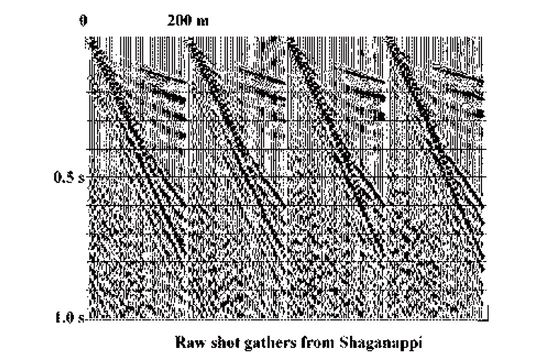
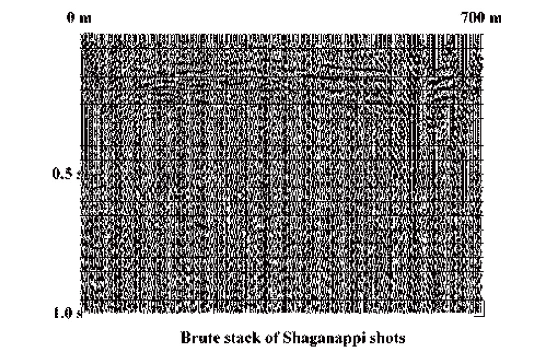
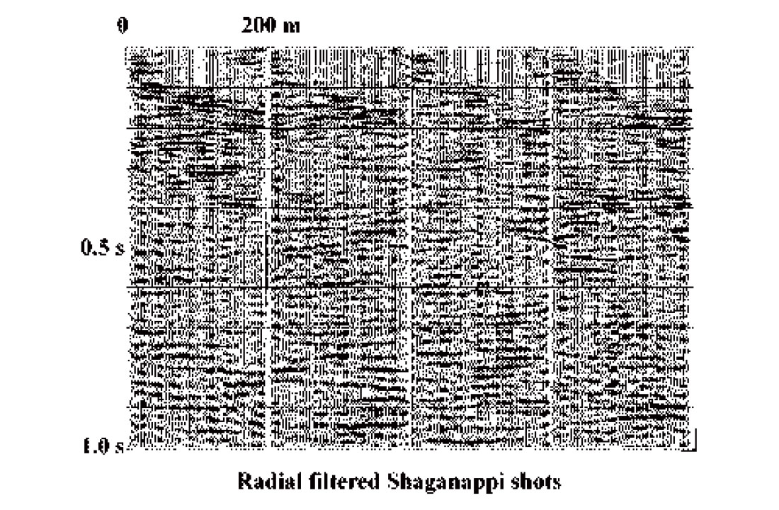
Figure 9 shows the shot gathers of Figure 7 after a single R-T domain filter pass designed to attenuate the strongest noise mode on the records (airblast). While the improvement is significant (some legitimate reflection energy is now visible), further analysis reveals other linear noises that can be successfully attenuated with either a radial fan or dip filter. Several successive R-T filter passes yield the records in Figure 10, on which many reflections are evident. The stack in Figure 11 shows the improved image obtained with these heavily filtered gathers. This image now contains very little mis-stacked noise and is consistent with the known shallow geology of the region (recent fluvial and glacial deposits).

Wavefield separation

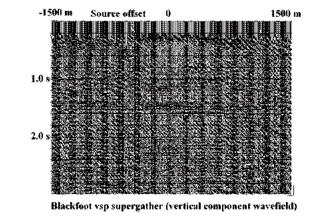
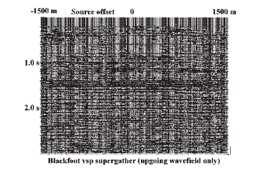
Coherent noise attenuation is merely a specific type of wavefield 3-C walk-away VSP survey at the Blackfoot field. Because this particular survey has only a small number of receiver levels in the borehole, wavefield separation can be made more effective by combining individual source gathers into a single supergather to increase event coherence length. Supergather events can be subsequently linearized and aligned by applying an approximate normal moveout (NMO) to correct for source-borehole offset and linear moveout (LMO) to correct for receiver depth. The supergather, with linear events coherent across most of the gather, can be filtered with a succession of R-T dip filters to sequentially suppress undesired wavefield components.

Figure 12 is the initial supergather for the vertical component of this VSP, Figure 13 is the NMO and LMO corrected supergather, and Figure 14 is the desired upgoing reflection wavefield. This supergather can now be decomposed into its original source gathers, and the upgoing events imaged using whatever technique is considered appropriate.

Regularization and other grid operations

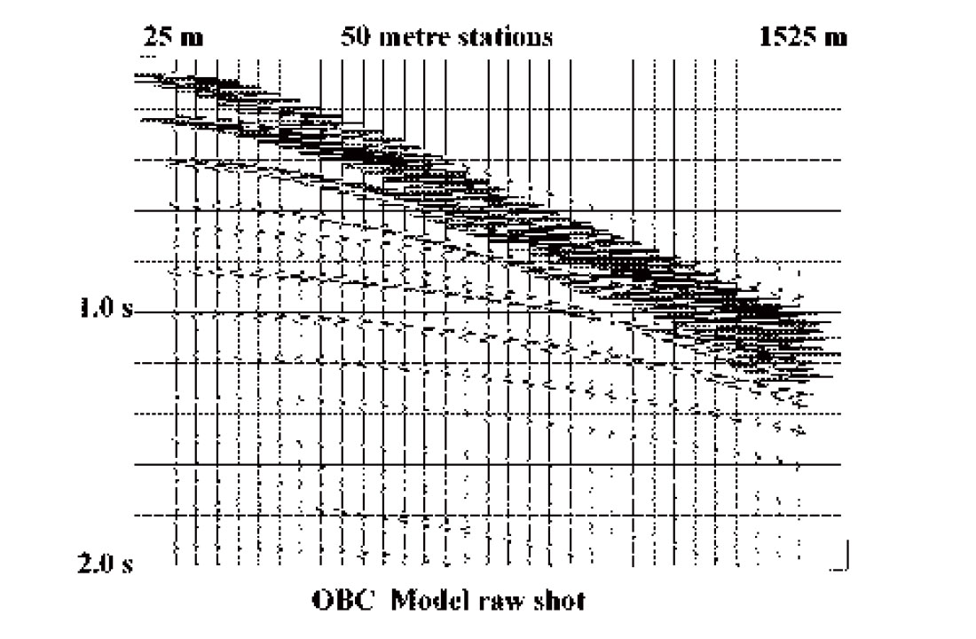
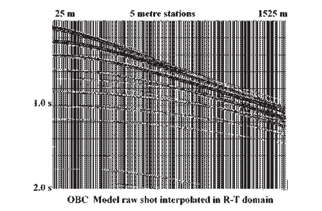
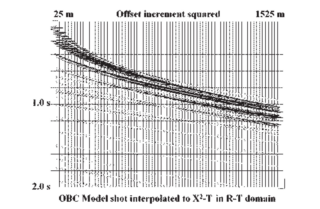
As an integral part of the R-T transform and its inverse, interpolation, per se, can also be one of its useful functions. Most implementations of the R-T transform have no restriction on the regularity of the X co-ordinate values of the input X-T panel; indeed one of the attractive features of the transform is that it uses whatever X values are present. To regularize the X values, however, it is only necessary to discard the original co-ordinates from the input trace headers and to supply a new set for the inverse radial transform. The new values can be uniformly spaced or non-linearly incremented, if desired. Furthermore, if the original X increment is too coarse or too fine, this can be changed as well. The only requirements for using the radial transform and its inverse for this re-mapping of the X-T domain are that all the new offset (X) values fall within the range of the values on the original X-T panel, and that events on the input panel are not significantly spatially aliased. Even aliased events can sometimes be accommodated, however, by applying partial moveout, either hyperbolic or linear, to the data before the R-T transform. To illustrate re-gridding of gathers, Figure 15 is a synthetic shot gather generated by Brian Hoffe of CREWES to simulate OBC data off the east coast of Canada. The slower events on the gather are significantly aliased due to the 50 metre station spacing. Nevertheless, by judiciously applying partial NMO (enough to remove the aliasing of the water-borne events without introducing significant aliasing into the faster reflection events), the gather can be interpolated to a simulated 5 metre station spacing as in Figure 16. By substituting quadratic offsets into the output trace headers, the X-T panel can, instead, be converted to X²-T, as in Figure 17. Data fidelity can be preserved in processes like this by carefully choosing the interpolation method and by keeping the disparity between X increment size in the input and output X-T domains relatively small (unlike the example).

Sea-floor rotation

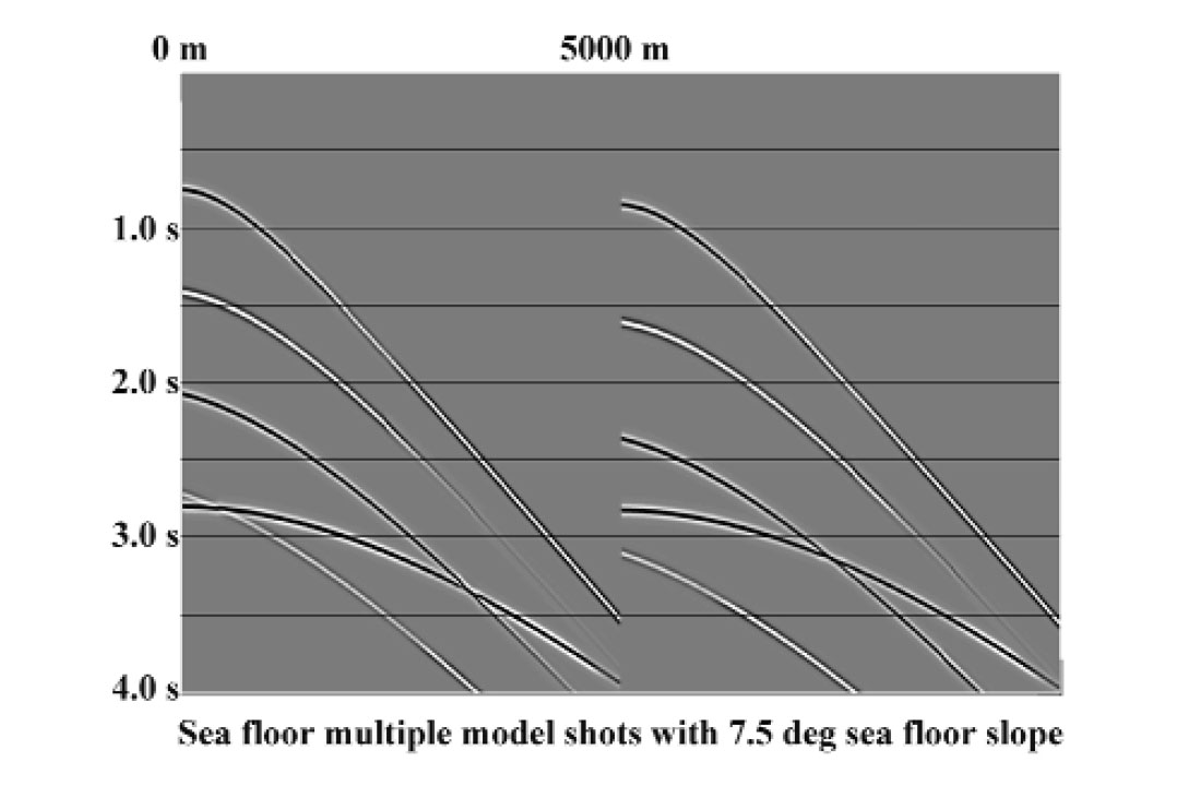
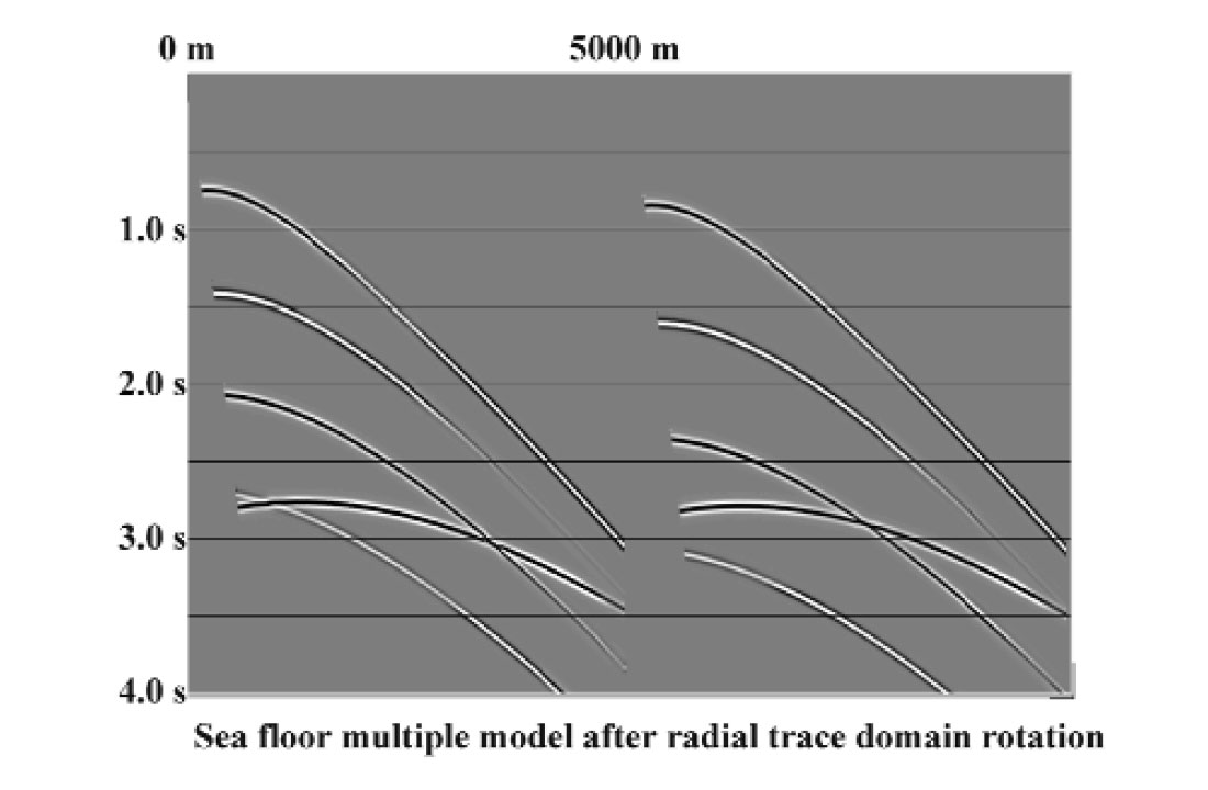
Simple sea-floor multiples have been attenuated in the R-T domain ever since this application was first demonstrated by Taner (1980). The favourable geometric relationships imposed by the R-T transform only hold for a flat-lying sea-floor, however, and subsequent development has been aimed at the problem of multiples from a sloping sea-floor. Lamont et al (1999) show how to deal with this problem by applying a dip-corrected moveout to primary and multiples. Another approach can be based on the properties of the R-T transform, without resorting to NMO correction with its attendant waveform distortion. A specialised R-T transform whose trace trajectories correspond to circular arcs in X-T can be used to capture and rotate the sea-floor primary and its multiples to approximate a flat sea-floor orientation. Figure 18 illustrates two simulated marine source gathers created by Pat Daley of CREWES for a 7.5 degree sloping sea-floor. The sea floor slope is evident in the limbs of the sea-floor multiples, which are steeper than they would be for a flat sea-floor. Figure 19 shows the result of rotating the shot gather in Figure 18 in the radial trace domain using circular radial traces. The timing irregularity due to sea-floor slope has been largely removed, and predictive multiple attenuation can now be more effectively applied to these gathers.

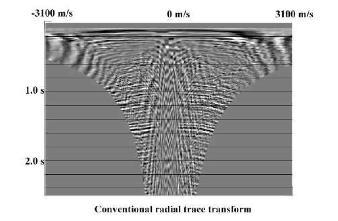
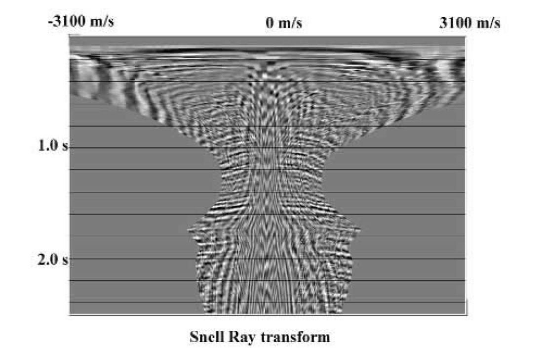
Snell-ray transform

Like the radial trace transform itself, the concept of the Snell-ray transform was introduced by the Stanford Exploration Project in connection with migration and imaging procedures (Ottolini, 1987). The Snell-ray transform differs from the standard R-T transform in that instead of using linear trajectories to gather wavefield amplitudes from the input X-T panel, the Snell-ray transform uses trajectories which obey Snell’s Law at every boundary marking a velocity change. Such radial traces, when sorted into panels of constant takeoff angle may prove useful in studies of amplitude versus angle (AVA). To illustrate the Snell-ray transform, Figure 20 contains a standard radial trace transform of a generic shot gather, while Figure 21 shows the equivalent Snell-ray transform, created using interval velocities consistent with the stacking velocity function for this line.

Radial trace transform continue

The few applications shown here may help to re-awaken interest in the versatile and under-used R-T transform. It should be remarked, however, that the radial trace transform is only one of a general class of mapping transforms (NMO-correction and CDP-mapping of VSP data are two other familiar ones). It may well prove worthwhile to reconsider other mapping transforms which might facilitate various aspects of the data enhancement and imaging techniques that form such a large part of geophysical practice today.

Acknowledgements

The author wishes to acknowledge the sponsors and staff of CREWES for support; Brian Hoffe and Pat Daley for synthetic models used in this work.