Results from diverse fracture analysis methodologies: consistent, contradictory, or complementary?

We examine four independent approaches to fracture detection using surface-seismic data. Fundamental algorithmic properties and limitations are studied in an attempt to explain observed differences between the attributes generated from the various approaches. Real data examples are presented, including one which demonstrates simultaneous analysis of all four techniques and which reinforces our belief that fracture characterization benefits from consideration of diverse attributes.

Introduction

Fracture estimation via analysis of surface-seismic data is enjoying increasing use in resource play development, and there are four approaches in common use today. The first and second of these examine amplitude and traveltime changes on wide azimuth P wave data (azimuthal AVO and azimuthal NMO approaches, respectively-- often termed “AVAZ” and “VVAZ”), while the third of these examines shear wave splitting on wide azimuth converted wave data (shear wave splitting or “SWS”). The fourth technique, volumetric curvature analysis, quantifies changes in reflector shapes on poststack volumes. Despite the increasing popularity of these techniques, dissenting opinions exist regarding their efficacy. Some workers claim good results in most cases, while others say the techniques never work and have been oversold. Such strong polarization of opinion obviously underscores our industry’s need to better answer the question of how well these techniques are working in practice.

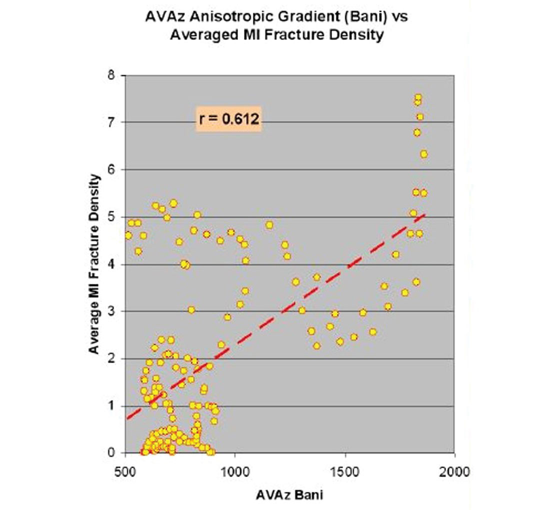
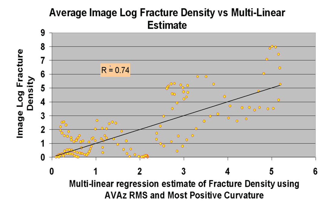
Despite the urgency surrounding the question, its answer has not yet been fully revealed. This is because the answer requires a substantial wellbore verification effort which, to date, has been conspicuously lacking. There are a few notable exceptions to this statement, as ground-truthing studies are beginning to emerge in the literature (e.g., Narhari et –., 2009; Jianming et al., 2009; Hunt et al., 2010; Treadgold et al., 2011; Sena et al., 2011). While all of these papers document some successful examples of usage, one of them objectively correlates estimated fracture densities with FMI data from horizontal wells over a significant spatial area. Specifically, the correlations of Hunt et al. (2010) between FMI fracture density and surface seismic attributes show some interesting characteristics. Figure 1, excerpted from their paper, shows a crossplot between FMI log fracture density and a fracture intensity attribute derived from AVAZ analysis. Although the crossplot trend suggests some degree of meaningful relationship between the attribute and the fracture intensity measured in the wellbore, the amount of scatter is, in the words of the article, “concerning”. The authors cite several possible reasons for the large (and peculiarly shaped) scatter, including noise, violation of underlying assumptions in attribute generation, and spatial scale disparities in measurement. They also advocate using multiple fracture predictors in order to reduce uncertainty. Figure 2 shows a similar crossplot to Figure 1, except that data from both AVAZ and curvature have been incorporated into the regression analysis. Note the improved correlation between this composite surface seismic attribute and the FMI data, an observation which supports their recommendation.

Combining multiple attributes into a single analysis is certainly a good idea – and indeed is the tack recommended in the present paper – but experience has shown that fracture maps generated by different techniques often show poor correlation. In their webcast, Hunt et al. (2011a) show numerous correlations between various kinds of fracture predicting attributes over several different data populations. The correlation coefficients were occasionally high over specific areas of interest, but typically became poor for very large unbiased data populations of up to 50,000 data samples. Interestingly, the correlation coefficients were always statistically significant despite being low (in the 0.2 to 0.3 range for the large populations). This level of correlation between AVAZ and most positive curvature was also observed in the Hunt et al. (2012) CSEG Symposium talk on the Wilrich (to be published in the SEG’s Interpretation journal). A low but statistically significant correlation is very different from no correlation, and may conform to expectations. Such statistical behavior implies that there is a data relationship but that the relationship is compromised by other factors, factors which we attempt to explain in the body of this paper. Delbecq et al. (2013) address this same observation of low correlation in the case of the three azimuthally-based techniques (AVAZ/VVAZ/SWS), and they point out that a main reason for observed discrepancies is the fact that different approaches are measuring different anisotropic rock properties at different vertical scales. These explanations hopefully provide some amount of solace to an interpreter feeling confused and skeptical in the face a dearth of well validation and a host of inconsistent results.

Our position is that these various fracture techniques do indeed hold promise, but that algorithm complexity and limitations, noise, and subtleness of the fracture-induced responses can conspire to make the interpretation very challenging. Accordingly, we believe that optimal interpretation requires a thorough understanding of all the assumptions underlying the various methods. Furthermore, we share the belief expressed in Hunt et al. (2010) that reliability may be heightened through joint analysis of attributes generated by diverse techniques and we are particularly interested in combining results from all four approaches. In the first part of this paper we seek to provide the interpreter with a complete and easy-to-understand list of the assumptions underlying all four techniques. The second part of the paper focuses on data examples which draw on this heightened algorithmic understanding. We hope this work will improve confidence in interpretation and will help see us through this awkward waiting period as the much-needed ground-truthing information – which provides the ultimate answer as to which techniques work well in which regimes – slowly trickles in.

Key algorithmic characteristics and limitations

The four fracture detection methodologies are well-documented in the literature. The AVAZ technique studied in this paper is based on the work of Rüger (1998) and the VVAZ technique is based on the Zheng inversion (Zheng, 2006). The converted wave SWS technique follows the method outlined by Li and Grossman (2012) and the curvature algorithm is discussed in Chopra and Marfurt (2011). The theory described in these references gives rise to many algorithmic limitations which we review below.

Data quality and noise issues

All three prestack techniques are sensitive to noise and to the effects of sparse spatial sampling. Although the advent of 5D interpolation has helped mitigate issues related to imperfect sampling, the field acquisition must still possess a sufficiently rich distribution of offsets and azimuths to allow the interpolation to identify multi-dimensional coherent signal trends. Strong noise, both random and linear, can lead to poor results in the case of all three techniques. AVAZ in particular requires an AVO compliant processing flow which can heighten sensitivity to noise. Also, azimuth-dependent linear noise and/or multiples may leak into the final migrated common offset vector ensembles which form the input to AVAZ and VVAZ. Well-known imaging issues in converted wave processing (low signal-to-noise, lack of high frequency content, large statics) may adversely affect SWS success. By contrast, the curvature approach is more robust with respect to noise and sampling issues because it is a poststack technique.

Data Resolution Discrepancies

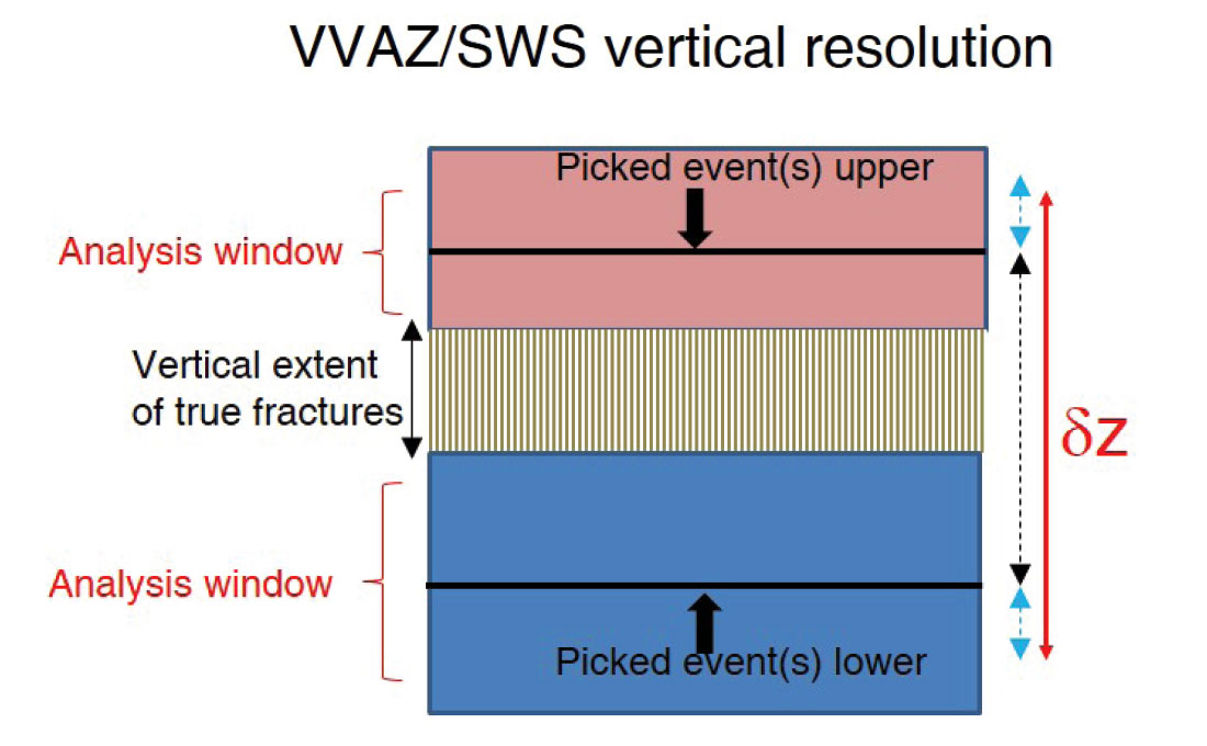
The fact that the four approaches carry inherent differences in resolution can lead to significant differences in the computed attribute maps. Both AVAZ and curvature measure properties at the seismic reflector, and therefore standard reflection processing resolution paradigms apply (i.e., lateral and vertical resolution ≈ λ/4 – note that both curvature and AVAZ analyses are typically performed after migration). By contrast both VVAZ and SWS are layer-based, rather than interface, techniques, a fact that has important implications for their resolution characteristics. A VVAZ layer is defined explicitly by picking top and base of the package of interest while a SWS layer is defined implicitly through a layer stripping process; in either case vertical resolution, δz, is governed largely by the 2-way-time-thickness of the layer under analysis (black dashed arrow, Figure 3) with a further limitation brought on by the size of the analysis window used to measure the azimuthally-variable traveltime distortions (blue dashed arrows, Figure 3). In practice a representative value might be δz =100 m for Western Canadian plains data, corresponding roughly to 100 ms and 150 ms PP and PS time, respectively.

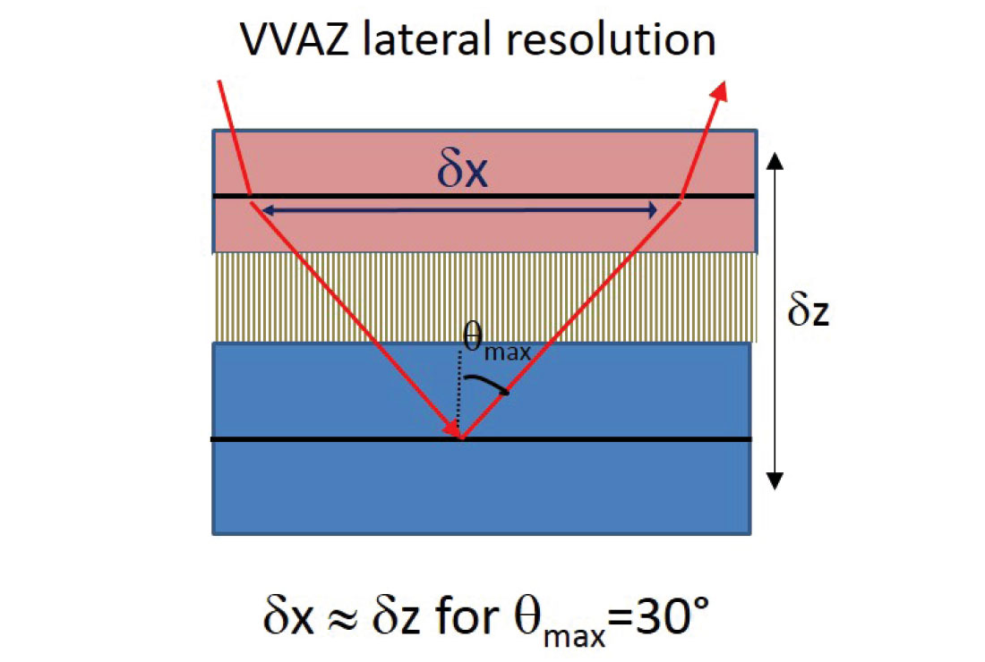
Lateral resolution is a somewhat murky topic for both VVAZ and SWS. In the case of the Zheng inversion (i.e., VVAZ), it is likely governed by the horizontal smear within the target layer of the various ray segments swept out by the incident angles sampled in each migrated gather as shown in Figure 4 (a typical range is 0° to 30°, and a simple geometric argument suggests a resolution limit equal to 2*layer_thickness* tan(30)≈ δz ). In the SWS case, the topic is complicated by the fact that the analysis is typically performed on unmigrated data (although Simmons (2009) shows a migrated-domain SWS example) for which the Fresnel zone has not yet been collapsed. We believe that lateral resolution is likely controlled by the maximum of the Fresnel zone and the asymptotic conversion point (ACP) supergather size (a representative value might be 300 m). Despite our struggle to precisely quantify lateral resolution, we are confident in asserting that VVAZ and SWS techniques yield similar resolution (both lateral and vertical), and moreover that this resolution is inferior to that associated with the AVAZ and curvature approaches.

Lateral heterogeneity ambiguity for VVAZ

Jenner (2009; 2010) shows how isotropic lateral velocity anomalies in the overburden can create phantom VVAZ responses which masquerade as anisotropy. It is unlikely that such false positives would be generated for the other two azimuthal approaches, and it is clear that the curvature approach would not suffer from this problem.

AVAZ reflection interface assumptions

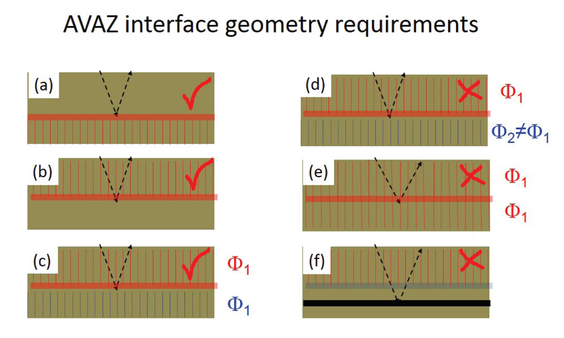
The underlying AVAZ theory imposes stringent requirements on the types of reflection events which admit accurate inversion. Specifically the theory assumes an isotropic layer overlying an HTI layer (HTI defined below), or vice-versa, and it also includes the case of two HTI layers possessing identical fracture orientations with differing fracture intensities. These three “permissible” reflector configurations are shown in Figures 5 a, b, and c, respectively. It follows that AVAZ will produce erroneous results in the case of two abutting layers possessing differing fracture orientations (Figure 5d) and will generate a null (i.e., zero) response on a reflection generated by a purely isotropic property contrast (Figure 5e). Such a null response could be misleading if the surrounding lithology were to exhibit uniform anisotropy, especially if this were the only picked interface in the vicinity of this anisotropic layer, as it would suggest an absence of anisotropy. Even when the interface assumptions are satisfied, the AVAZ measurement may be distorted if the reflection event is weak or obscured by noise. By contrast, this same problem can be avoided for VVAZ and SWS techniques if the user is able to pick clean reflection events which lie a small distance outboard from the true layer of interest (the resulting degradation in vertical resolution may be offset by the benefits associated with inverting cleaner data). This situation is depicted in Figure 5f.

Rock physics considerations and orientation ambiguity

As discussed in Delbecq et al. (2013), the three prestack azimuthal methods measure different aspects of anisotropy. Curvature measurements differ fundamentally in their relationship to fractures (i.e., compared to any of these azimuthal approaches) as they involve considerations of stress, strain and brittleness instead of anisotropy. The fact that these attributes are all measuring different fracture “signatures” can help explain the differences observed in the output attributes. The AVAZ technique is sensitive to the contrast in two Thomsen parameters γ^(v) and δ^(v) (these describe layer-localized shear wave splitting and layer-localized P wave NMO velocity differences parallel and perpendicular to fractures, respectively) across an interface, while the VVAZ and SWS responses depend on δ^(v) alone and γ^(v) alone, respectively, within the layer of interest. Because these anisotropic measurements can be directly interpreted in terms of fracture orientation and intensity, all three azimuthal approaches may be considered as direct fracture indicators. By contrast, the poststack curvature technique is an indirect indicator, since an increase in curvature implies increased strain which may or may not imply fracturing, depending on the degree of brittleness of the rock. Hunt et al. (2011b) show the importance of considering rock properties alongside curvature in their creation of the stress-curvature attribute, which is essentially a scaling of curvature by Young’s modulus. This work has received some quantitative ground-truthing via vertical and lateral FMI data. The philosophy behind this effort is to improve indirect fracture indicators by considering several of them within a framework that is congruent with rock physics.

The AVAZ 90 degree orientation ambiguity is well documented (e.g., Zheng et al., 2004) and stems from the fact that the industry-standard Rüger equation is a small incident angle truncation of a higher order expression as discussed in Goodway et al. (2006). Note that a recent alternative AVAZ approach based on azimuthal Fourier analysis can overcome this orientation ambiguity (Downton et al., 2011). Although the Zheng inversion for VVAZ also suffers from a theoretical ambiguity in orientation angle, experience has shown that it may be resolved in most situations by making the geologically reasonable assumption of negativity of δ^\(v). The SWS technique does not suffer from this orientation ambiguity, as the fast shear wave is always polarized along fracture strike (or along the maximum horizontal stress direction, in the case of stress-induced anisotropy).

The HTI anisotropy assumption

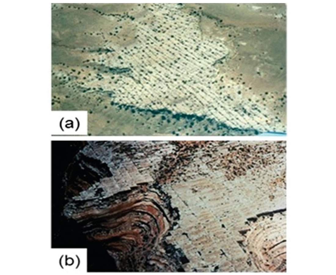
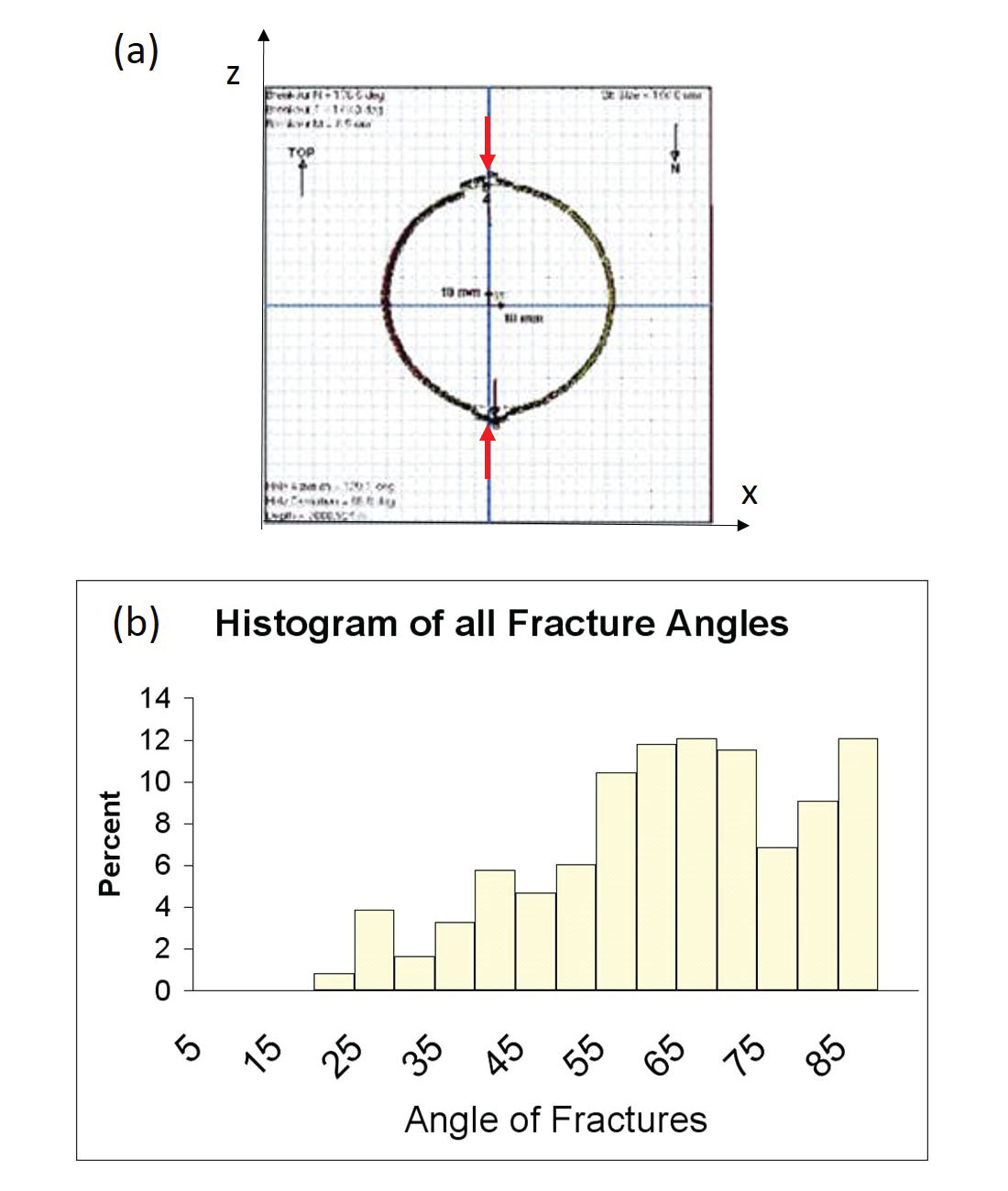
The AVAZ and VVAZ inversions are based on that class of anisotropy known as horizontal transverse isotropy (HTI). The HTI model assumes the existence of locally mono-oriented sets of vertical fractures. Unfortunately fracture sets in the real world don’t always conform to this simple configuration: Figure 6a shows a case where this single-orientation assumption appears to be satisfied while Figure 6b shows a case where it is clearly invalid. The assumption of fracture verticality also deserves some scrutiny. Figure 7a shows an image of borehole breakout for a horizontal well drilled into the Cardium formation in central Alberta. The vertical direction of breakout (red arrows) suggests that the maximum compressive stress is in the horizontal plane, which in turn implies that the attitude of associated compressive fractures would not be near-vertical. This latter suggestion is borne out by the FMI log data whose associated fracture attitudes are displayed in a histogram in Figure 7b. The histogram shows that the measured fracture attitudes indeed show significant departure from vertical and therefore from the HTI model. Though not shown here, a similar analysis carried out in the Nordegg formation – where an AVAZ analysis showed promising results – revealed near vertical fracture attitudes (Hunt et al, 2010).

Although we may still measure azimuthally varying AVO and/or velocity effects in cases where the fractures don’t conform to the HTI model, it would not be appropriate to relate the computed fracture intensity attribute to γ^(v) and δ^\(v) (nor to alternative formulations of HTI parameters), and the orientation estimate could not be related to a single fracture set. In the SWS case, various classes of anisotropy are known to induce fast and slow polarized shear waves, and although the HTI class gives rise to a particularly simple interpretation of SWS intensity and orientation, other interpretations exist for more complicated classes (Winterstein, 1999).

Real data examples

In this section we show two real data examples, each of which has produced results which are at once promising and perplexing. By applying our learnings about algorithmic characteristics and limitations to these case studies, we believe we are able to resolve some of the confusion in interpretation.

AVAZ/VVAZ example from central Alberta

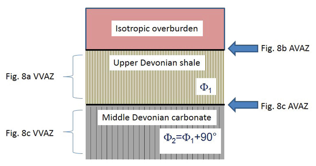
Figure 8a shows VVAZ intensity and orientation maps for an upper Devonian shale unit, and Figures 8b and 8d show the AVAZ intensity maps at top and base of the unit, respectively. While the VVAZ intensity map shows some correlation with the AVAZ map from the top-ofunit reflector, it reveals poor correlation with the AVAZ map from the base-of-unit reflector. Figure 8c shows the VVAZ map for the middle Devonian carbonate interval immediately underlying the interval of interest. Note that the orientations appear “flip-flopped” approximately 90 degrees in the zones of strong fracturing compared to the VVAZ image from the overlying unit in Fig. 8a. This orientation flip-flop was also observed on the FMI log from a nearby vertical well, suggesting that the VVAZ technique is giving reliable fracture orientation estimates. In light of the above discussion, it seems likely that the base-of-unit AVAZ map (Figure 8d) is unreliable because the Rüger equation is violated in the case of two abutting fractured layers with differing orientations (i.e., as per Figure 5d). This interpretation is shown in schematic form in Figure 9.

SWS/VVAZ/curvature/AVAZ example from Blackfoot 3D 3C data set, south-central Alberta

In this example we consider attributes generated by all four techniques. The data set under study, the Blackfoot 3D 3C data set from south-central Alberta, was chosen largely because it is one of the few publicly available 3D 3C data sets (note that fracture detection results are typically tightly guarded by companies). To our knowledge, this is the first-ever public showcasing of simultaneous use of all four fracture detection techniques. Unfortunately the geology in the survey area does not exhibit strong fracturing, nor do we have access to wellbore data such as FMI logs, so this data set is arguably not the best choice for such a demonstration. On the other hand, it does have a good signal-to-noise ratio, and has produced some interesting attribute maps as we will show below.

Figures 10a and 10b show the shear-wave splitting and P wave azimuthal velocity variation at a CMP/ACP location which exhibits some of the strongest anisotropic behavior across the entire survey. The tell-tale signs of anisotropy are present, but relatively faint compared to most data examples we encounter: specifically we note a small amount of sinusoidal wobble on events on the radial component of the PS limited-azimuth-stack and the presence of some amount of coherent signal on the transverse component (Figure 10a); also, we observe some sinusoidal wobble on far-offset events on the P wave COCA display (Figure 10b). Given our expectation of a lack of fracturing at depth, we chose to focus our efforts on characterizing the shallow stress-induced anisotropy. Stress-induced anisotropy arises when differential horizontal stress fields cause preferential alignment of very small-scale “micro-cracks” in the direction of maximum horizontal stress; such anisotropy need not involve the formation of fractures, which are generally manifest at larger, though still sub-seismic-wavelength, spatial scales.

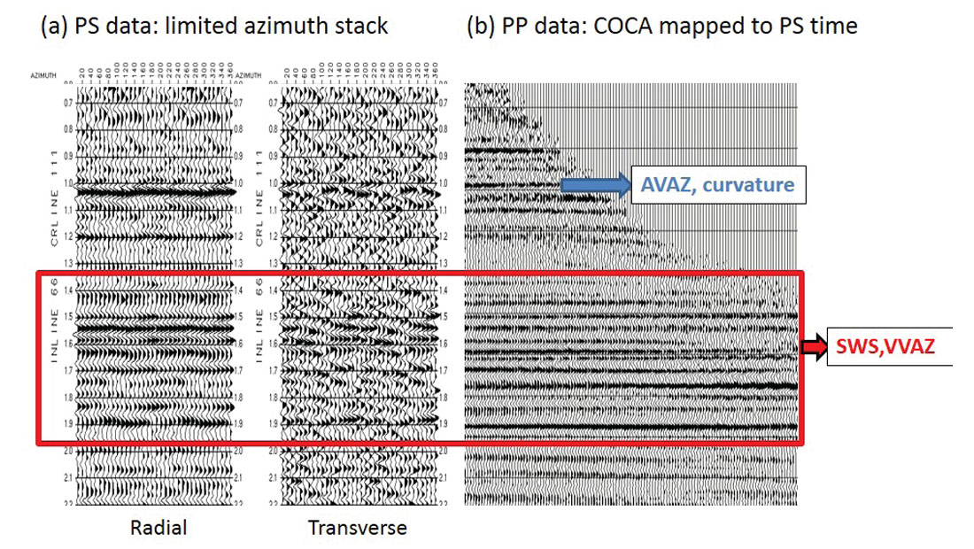
From our above discussion on resolution, we might anticipate one set of consistent attribute images from VVAZ and SWS, and a different set of consistent images from AVAZ and curvature. With this in mind, we chose our shear wave splitting analysis window to encompass the shallowest regionally stable reflector package (red box, Figure 10a), and then defined our VVAZ analysis window so that it captured the same data package on the PP section (red box, Figure 10b). In a similar fashion, we chose the shallowest regionally stable single reflector for both the AVAZ and curvature analysis (blue arrow, Figure 10b).

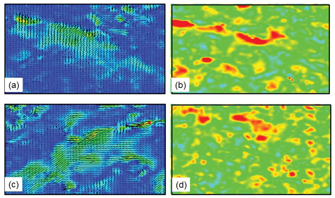
Figures 11a and 11b show the VVAZ and SWS fracture maps, respectively. There is a good deal of similarity in the long wavelength patterns (although we also observe some puzzling differences). We note with interest that both techniques are sensing an overall SW-NE orientation which is consistent with the dominant direction of maximum regional horizontal stress in the area. In short, we are encouraged by the similarity of the results and we believe the techniques have succeeded in capturing the long wavelength trends of the regional horizontal stress anisotropy. Our observation here is consistent with the work of Cary et al. (2010), who show a more impressive correlation between VVAZ and SWS attribute maps in the shallow section of a heavy oil data set, and also with the comments of Delbecq et al. (2013) who assert that SWS and VVAZ should capture information about regional stresses.

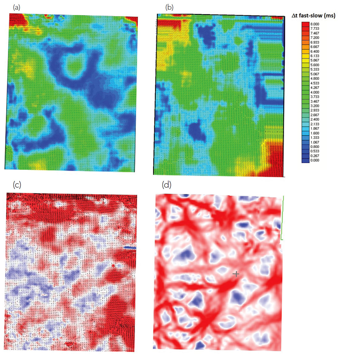
Figures 11c and 11d show the AVAZ and long-wavelength curvature maps extracted from the shallow horizon indicated by the blue arrow in Figure 10b. These two maps show very little correlation with the SWS and VVAZ maps (i.e., Figures 11a and 11b); also, aside from the presence of some common SW-NE linearly trending features, the maps in Figures 11c and 11d show little correlation to one another – this despite the theoretical suggestion that curvature and AVAZ should give similar results. We believe that our above discussion about algorithm characteristics provides an explanation for these puzzling observations. Given that we do not expect strong fracturing in this data area, it is likely that this particular reflection event does not represent a boundary between fractured and unfractured rock, and thus likely that neither AVAZ nor curvature are picking up a meaningful fracture response. As a corollary, it follows that any relatively strong anomalies that are present on the curvature map probably do not correspond to fractures (recall that strong curvature does not necessarily imply the presence of fractures). Of course such conjectures could only be validated via well control, but in the absence of such ground-truthing we feel that this interpretation is consistent with data observations, our understanding of algorithm limitations, and our a priori knowledge about the geology.

Summary

Various algorithmic limitations and characteristics may conspire to produce fracture maps which do not appear consistent; in the worstcase scenario of heavy violation of algorithmic assumptions, it is conceivable that such attributes may even appear contradictory. Equipped with a good understanding of algorithmic workings and relative pros and cons, we can often remove the confusion in interpretation, and in some cases may find that these diverse attribute maps contain complimentary information.

Acknowledgements

We acknowledge Richard Bale, a 3C expert whose witty alliteration at the podium at last year’s CSEG convention inspired us to include an altogether different set of 3C’s in the title of this paper. We thank Scott Cooper and John Lorenz of Fracture Studies for providing the fracture photographs as well as an anonymous data donor for allowing us to show certain fracture attribute maps. We thank Santonia Energy Inc. for allowing us to show the Cardium wellbore data and we thank CREWES for use of the Blackfoot data.