Pseudo Gamma Ray Volumes Estimated from Offset Seismic

Using seismic to explore for clastic reservoirs in the Western Canada Sedimentary Basin is often difficult due to the inability to distinguish between interbedded sand and shale lithologies using acoustic impedance. The problem is made even more difficult when the AVO response to sand-shale interfaces distorts the reflection amplitudes on a stacked section.

Geologists typically use a Gamma Ray log (or Vshale log derived from Gamma Ray) for lithology discrimination. Seismic, on the other hand, responds to changes in compressional velocity, shear velocity, and density.

The goal is to establish a relationship between gamma ray logs and the seismic logs (V_p, V_s, and Density) and then use this relationship to estimate the expected gamma ray response from seismic data.

A simple method to create a pseudo gamma ray log using dipole sonic and density logs is presented. The method is extended to the seismic domain and shown to be effective for interpreting sand-shale lithologies and for mapping net to gross sand-shale ratios within limitations imposed by the seismic bandwidth.

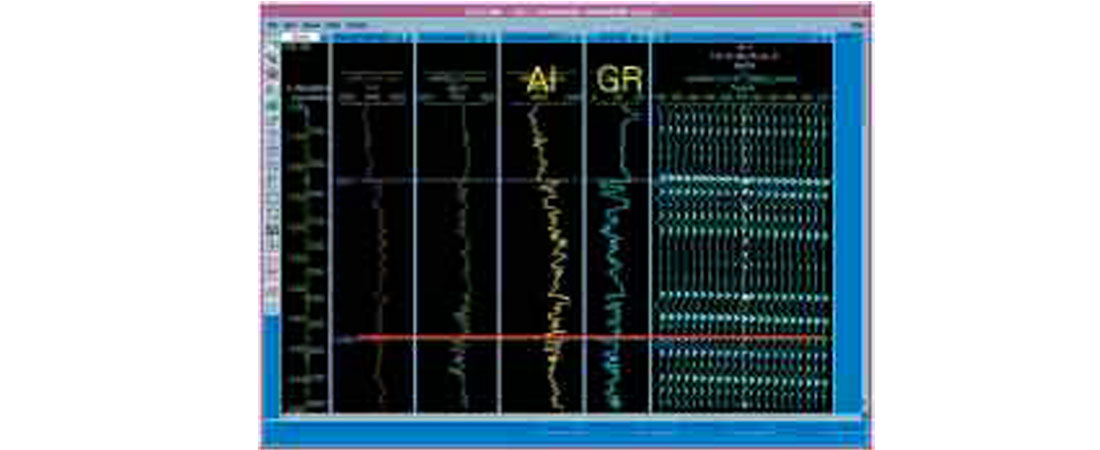
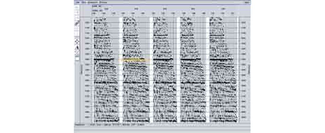
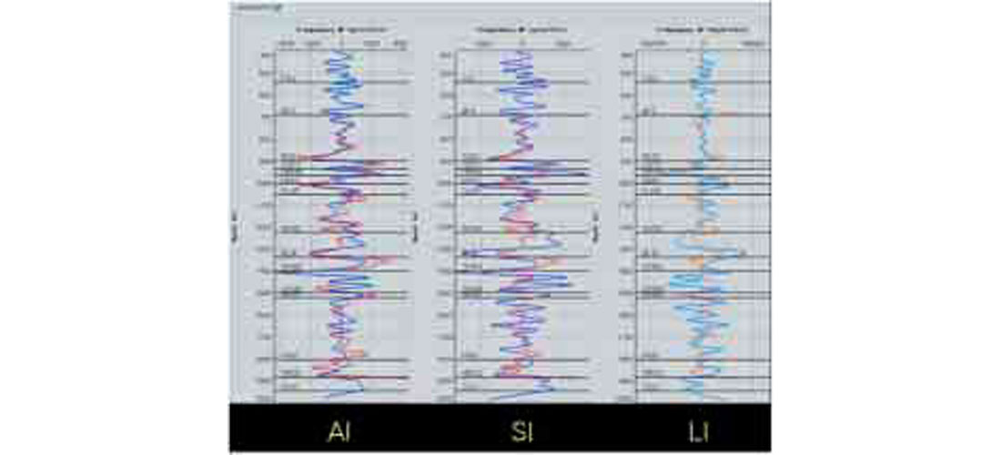
Figure 1 shows an example of the sand / shale interbedding problem in the lower Cretaceous of NEBC. The gamma ray curve (GR) identifies the clean sands but there is no obvious correlation to the top and base sands on the acoustic impedance log (AI). The corresponding seismic shows a relatively poor reflection that corresponds to the top of sand.

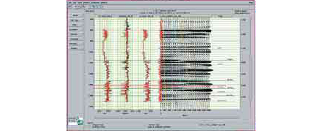
Figure 2 shows an example of the AVO response for the same well.

Note how in many cases the amplitudes actually change polarity across the model. The coloured lines on the model indicate the incidence angle, the yellow line on the left is 5 degrees and the brown line on the right is 45 degrees.

Creating a Pseudo Gamma Ray log from Seismic logs

Just as acoustic impedance (AI) is defined as density (ρ) times compressional velocity (V_p), shear impedance (SI) can be defined as density times shear velocity (V_s).

AI and SI logs can be calculated for any well with V_p, V_s, and density logs and then combined in a simple way to give a reasonable estimate of the associated gamma ray curve for a consolidated clastic section. This estimated Pseudo Gamma Ray log is equivalent to the EI curve optimized for lithology as described by Whitcombe, Connolly, and Redshaw.

Figures 3 through 8 provide a visual demonstration of the process for estimating the Pseudo Gamma Ray log using AI and SI logs calculated for a well in the lower Cretaceous.

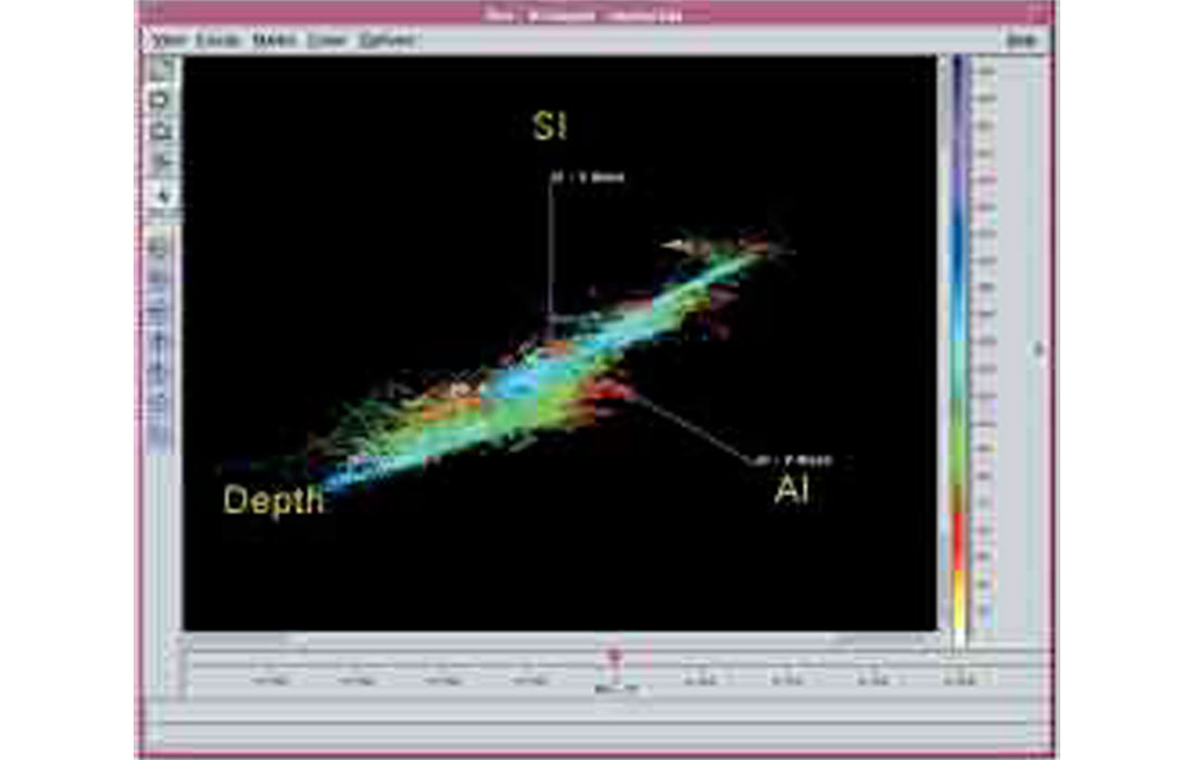
Figure 3 shows a three dimensional crossplot with the axis corresponding to AI, SI and measured depth. The data points are coloured based on the corresponding gamma ray values with low API values (clean sands) represented by the warm colours (red and yellows) and high API values (shales) represented by the cool colours (green and blue).

Figure 4 shows the same three dimensional space rotated until the SI axis comes out of the page. The result is a projection in AI / Depth space which is nothing more than the AI log displayed as a series of points. Note, in the lower portion of the well the sand and shale zones are heavily intertwined.

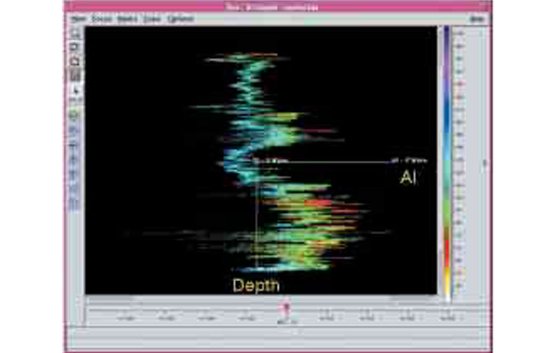
Figure 5 shows the space rotated around until the AI axis is perpendicular to the page which results in a plot of the SI log.

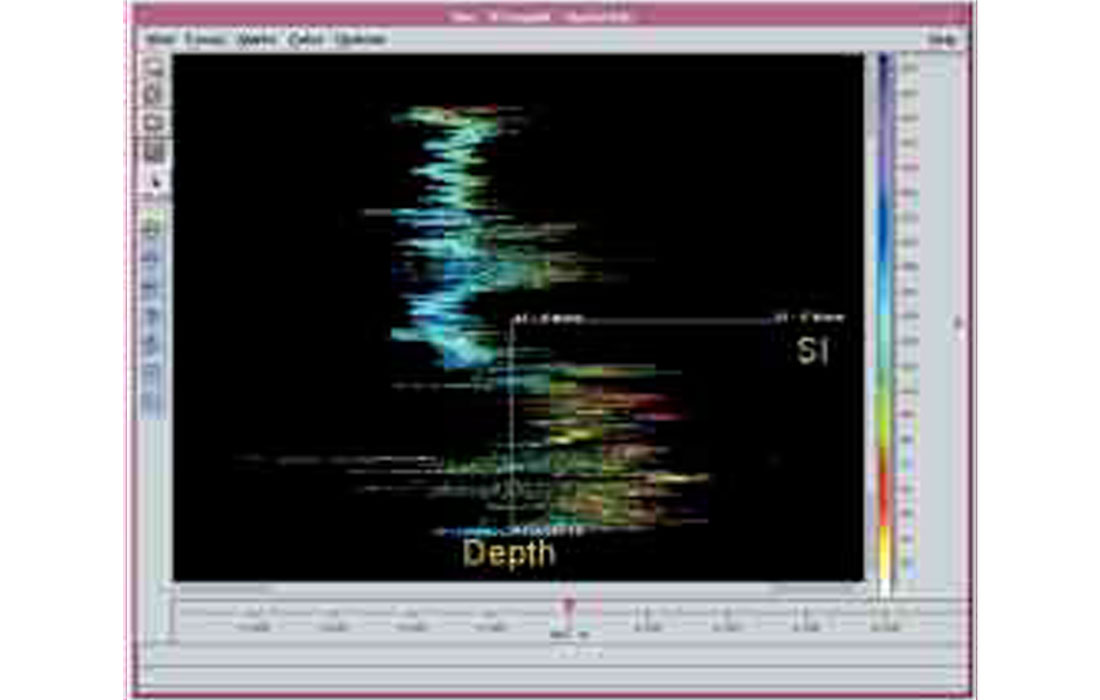
Figure 6 shows the space rotated once more until the depth axis is perpendicular to the page which gives us an AI / SI crossplot. Note how in this space the sands and shales tend to separate into two almost parallel trends.

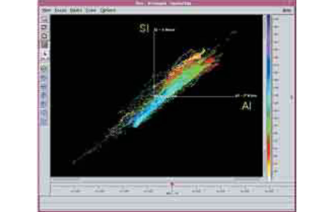
Figure 7 shows the space rotated around the depth axis until the sand and shale trends are approximately vertical. The resultant horizontal axis is what we will call our Lithology Impedance (LI) or Pseudo Gamma Ray axis.

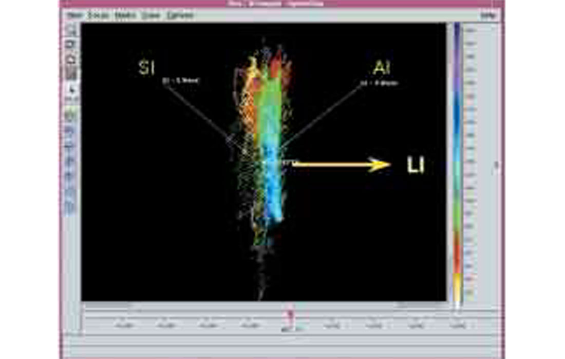
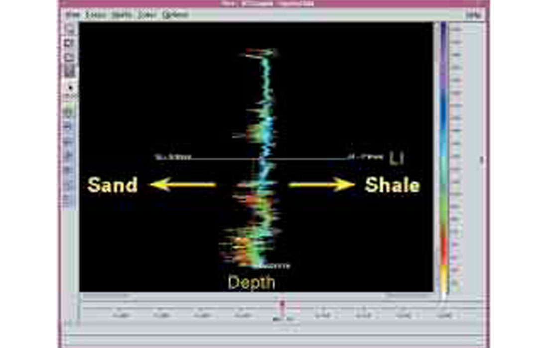
Figure 8 shows the space rotated one last time around the new LI axis until the depth axis is once again vertical. The resultant projection shows the LI values as a function of depth and this is our new Pseudo Gamma curve. Note, the sands tend to separate to the left and the shales to the right in a similar fashion to a gamma ray log.

This visual display is convenient to provide insight into the process but does not provide a particularly useful methodology for a practical application of the process.

Mathematically, the process of rotating the derived AI and SI logs about the depth axis through an angle θ (theta) and projecting the result onto the new horizontal axis is equivalent to the following equation.

LI(z) = AI(z) cos(θ) - SI(z) sin(θ)

where

In practice, a more rigourous approach is to calculate the LI curve for a range of angles and crosscorrelate the result with the gamma ray log over the zone of interest to determine the optimum angle.

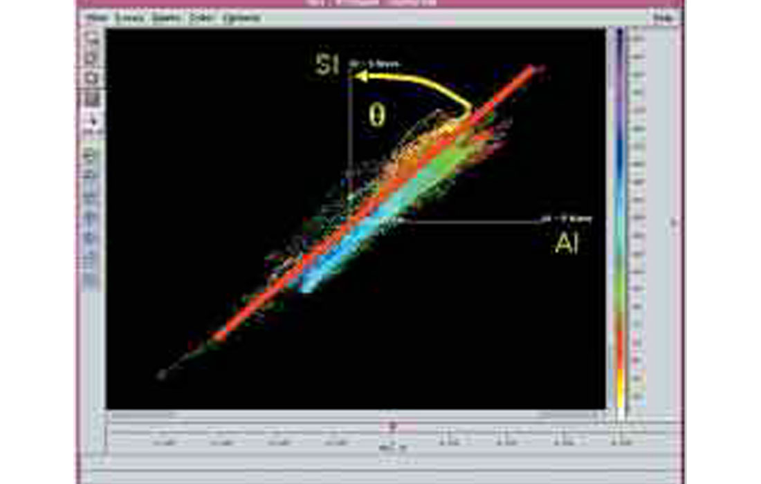
Figure 10 shows the results of rotating two wells through a range of 40 to 90 degrees and the resultant crosscorrelation values. The vertical black line at 70 degrees is the average best fit angle which resulted in a maximum crosscorrelation of .80 and .82.

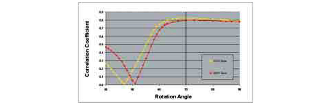
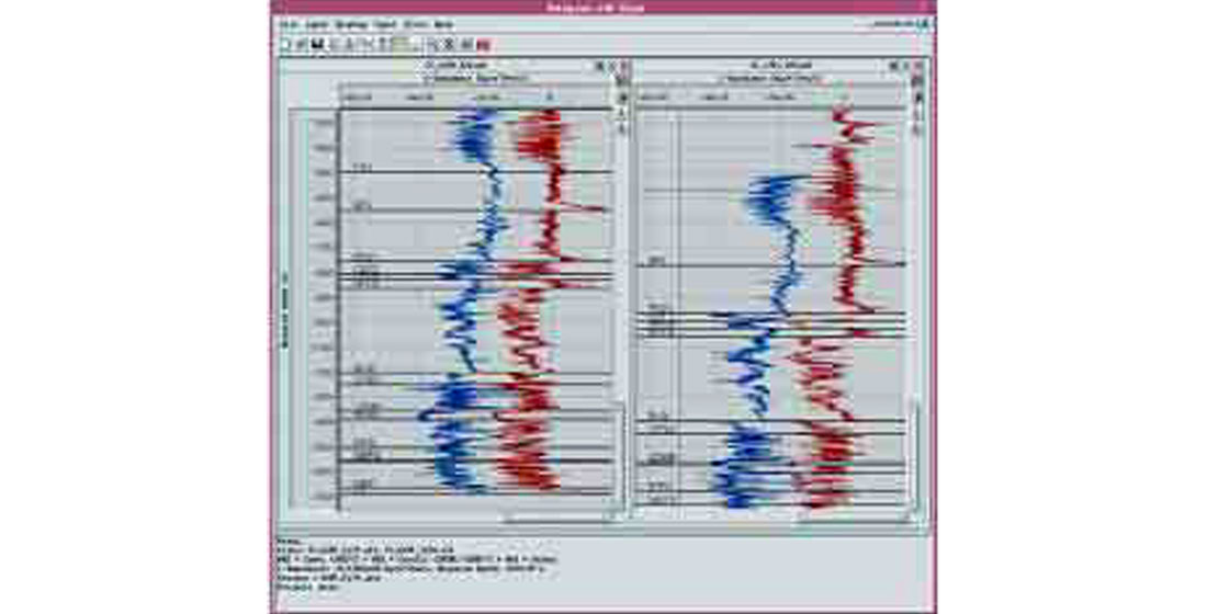
Figure 11 shows the result corresponding to a Pseudo Gamma Ray curve generated with a 70° rotation. The line in green is the actual gamma ray curve while the line in purple is the estimated curve. Note the particularly good fit over the Paddy/Cadotte zone (expanded on the right side of the figure) which was the zone of interest and the interval for which the crosscorrelation was maximized.

Pseudo Gamma Ray from Model Seismic

Having established a reasonable estimate of a gamma ray curve can be created from acoustic and shear impedance curves, we now demonstrate that an equivalent process can be applied to offset seismic data.

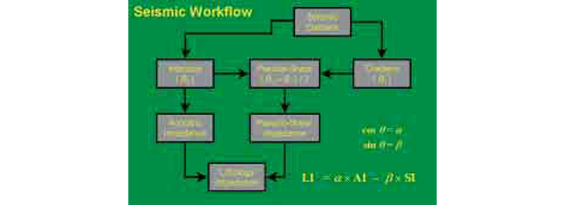
Figure 12 summarizes the workflow used to create a Pseudo Gamma Ray log from offset seismic gathers.

1. The CDP gathers are used to estimate Intercept (B0) and Gradient (B1) volumes.
2. Based on the conventional approximation for amplitude versus offset, shear reflectivity can be estimated as (B0-B1)/2.
3. The Intercept is an estimate of zero offset reflectivity and can be inverted to get an estimate of Acoustic Impedance.
4. The Pseudo Shear reflectivity estimated from the Intercept and Gradient can be inverted for an estimate of Shear Impedance.
5. The Acoustic and Shear Impedance volumes can be combined in the same manner as the AI and SI logs to create a Lithology Impedance (Pseudo Gamma Ray) volume.

To test the work flow, a series of logs was created into which wedges of sand were inserted using log responses from known sand intervals of nearby wells. For each log, an artificial gather was created with a bandwidth similar to that of the available seismic data. The gathers were processed using the work flow and the same processes that would be applied to real data.

Figure 13 shows the gamma ray curves for the modified logs with the sand intervals identified by the yellow boxes. Equivalent V_p, V_s, and density curves were also created.

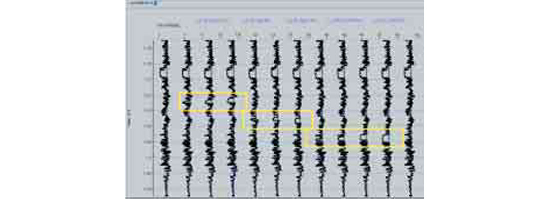
Figure 14 shows the Intercept traces calculated from the gathers. The boxes indicate the location of the sand bodies but the response from the sand is very subtle.

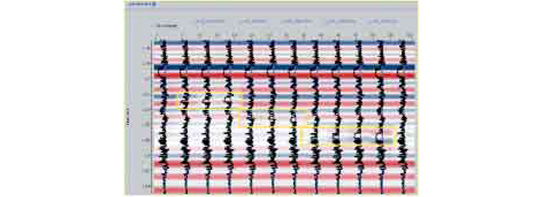
Figure 15 shows the result of inverting the intercept section. The sand bodies create more obvious differences on this section but it is not clear that the types of anomalies created would be identified as sand bodies.

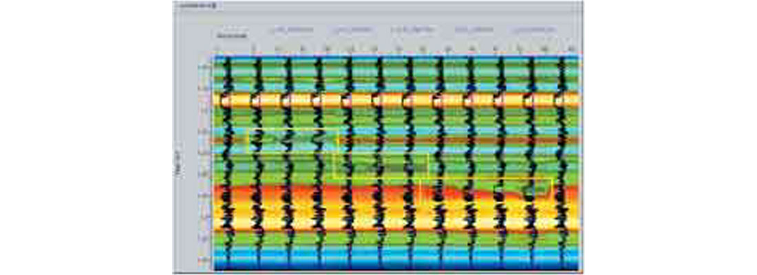
Figure 16 shows the final LI or Pseudo Gamma Ray section which shows very obvious anomalies at the location of the uppermost and lowermost sand and a less obvious anomaly for the middle sand.

While the LI section appears to identify the sand zones most clearly, the figure also gives some insight into the limitations of the process due to the bandlimited nature of the seismic data. In particular, it should be noted that zones away from those that were modified also show changes.

Pseudo Gamma Ray from Real Seismic

Having determined that there is hope for identifying sand zones using the Pseudo Gamma Ray volume, the workflow was applied to a real 3D volume.

The first step is to calculate the Intercept and Gradient from the offset gathers.

Figure 17 shows a typical flattened gather. For a given time sample (as indicated by the horizontal yellow line on the gather), the amplitudes from each trace in the gather are extracted.

AVO theory predicts that the change of amplitude with offset is approximately linear if plotted as a function of sin²(θ) where θ is the angle of incidence at the reflection boundary.

For each amplitude value from the gather the associated incidence angle θ is estimated based on the velocity function used to process the seismic data. The amplitudes can be plotted as a function of sin²(θ) as shown in Figure 18, and a best fit line calculated using linear regression.

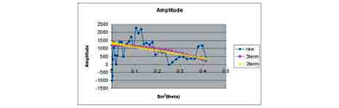
Calculating the best fit line for every sample from every trace results in Intercept and Gradient volumes which can be displayed like any other seismic volume.

AVO theory also predicts that shear reflectivity can be estimated from B0 and B1 using the simple calculation (B0 - B1) / 2.

Performing this calculation for every sample from every trace of the B0 and B1 volumes results in a shear reflectivity volume.

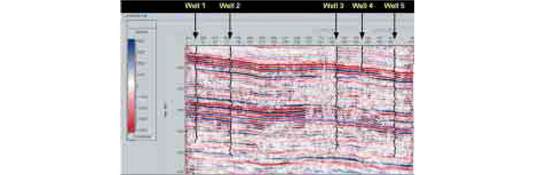
The quality of the inversion is highly dependent on an accurate estimate of the wavelet in the data. For this study, the wavelet was estimated based on two well ties (Well 2 and Well 5 on the plots above).

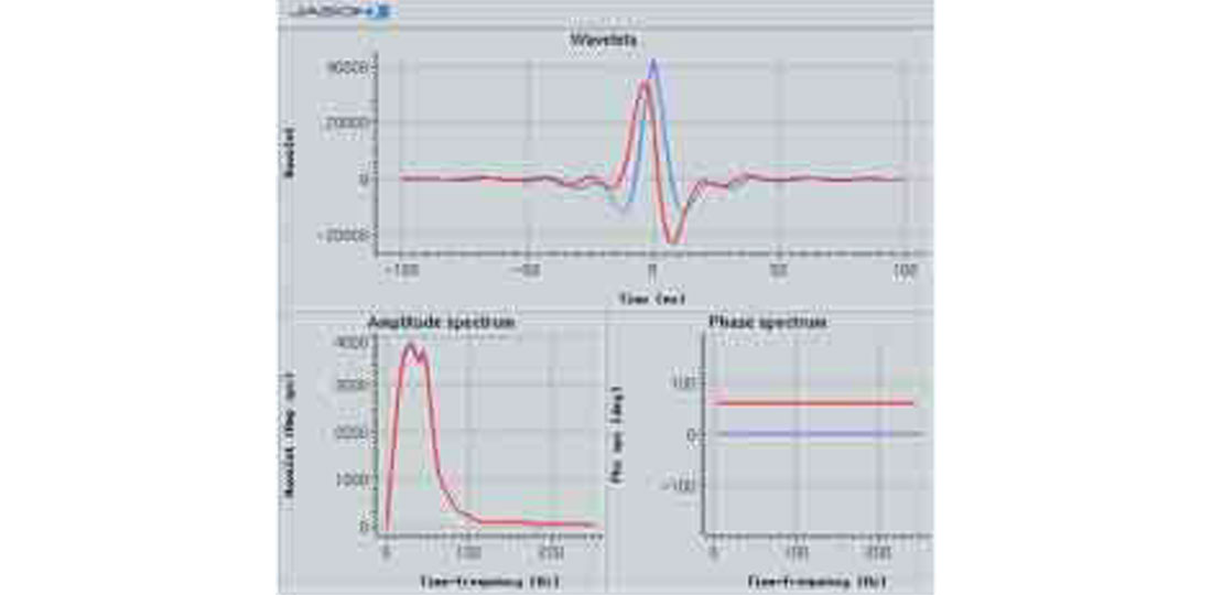
Figure 22 shows the estimated constant phase wavelet used for the inversions.

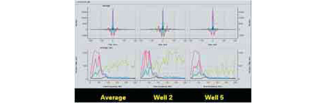
An important step in wavelet estimation for generating confidence is quality control. Figure 23 is a QC plot provided by the wavelet extraction software. The lower row of the plot is of primary interest. The green curves are the frequency spectra of the well reflectivity. The red curves are the spectra from the seismic. The light blue curve represents the error between the seismic spectra and the well spectra. The purple curves are the spectra of the estimated wavelet. The dark blue curve (which follows the well reflectivity curve over the bandwidth of the seismic) is the spectra of the output reflectivity from the inversion process. The black curve is the spectra of the error remaining after the inversion. If the wavelet estimate is good, the spectra of the output reflectivity will match the reflectivity of the well.

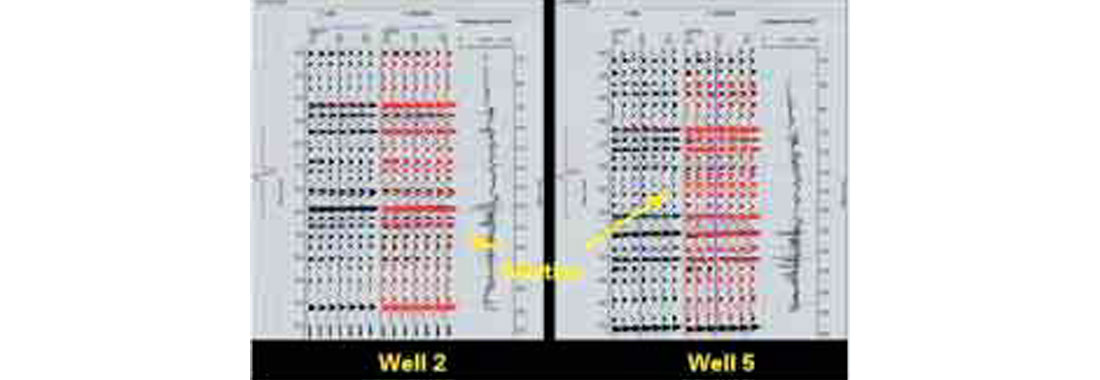
An alternate QC step is to use the estimated wavelet to create synthetics which should match the seismic at the well locations. Figure 24 shows the synthetics for the two wells used for the wavelet extraction process. The black traces are the actual zero offset reflectivity data, while the red traces are the synthetics generated using the estimated wavelet. Note that while the overall tie is extremely good, there are zones in both wells which have a fairly significant mistie. It will be seen that these misties will remain after the inversion process.

Once a reliable wavelet has been estimated it is used to invert the Intercept (B0) volume to get an estimate of Acoustic Impedance and to invert the Pseudo Shear Reflectivity to get an estimate of Shear Impedance.

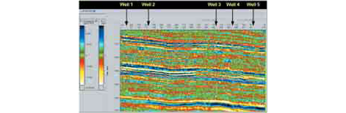
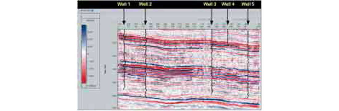
Figure 25 shows the bandlimited Acoustic Impedance section created using Jason’s Sparse Spike Inversion algorithm with no constraints. Any other inversion process could also theoretically be used for this step. Superimposed on the section are the acoustic impedance logs of the 5 well ties bandpassed to match the frequency content of the seismic and scaled so that the same colour bar could be used. The well ties are so good that they are extremely difficult to pick out from the background seismic.

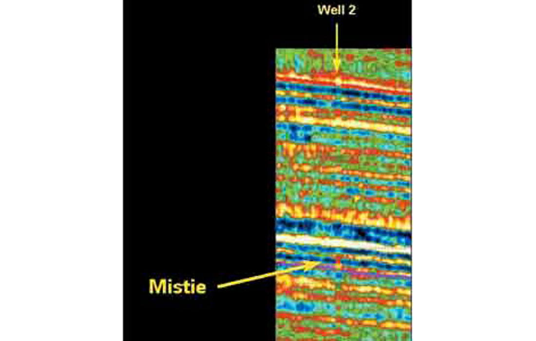
Figure 26 is a blowup of the tie at Well 2. Note that while the tie is good, the zone where the mistie occurred on the reflectivity data does not have a good tie on the impedance data.

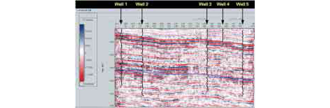
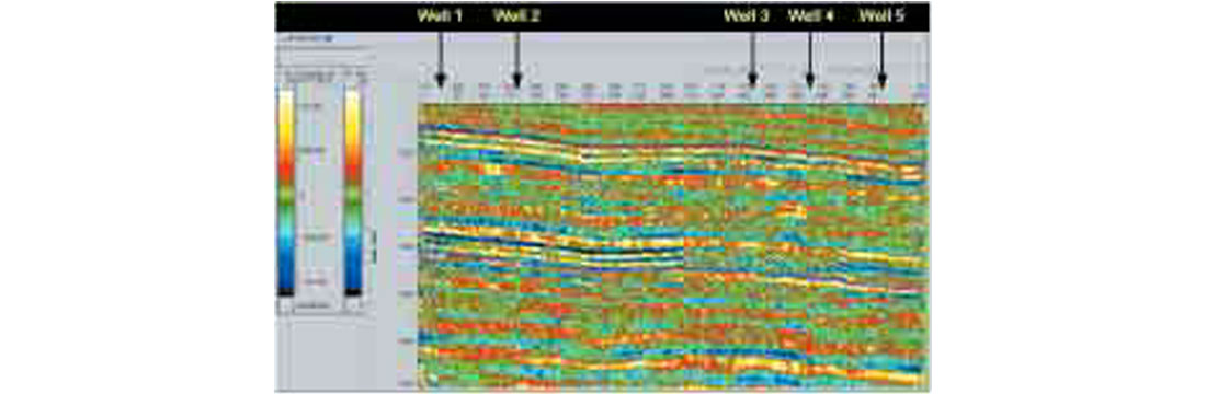
Figure 27 is the Pseudo-Shear Impedance section with the bandpassed Shear Impedance logs superimposed at the tie locations.

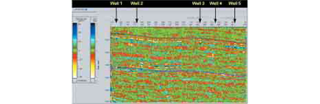
The impedance volumes can be combined using the same simple linear combination defined in equation (1) to create a Pseudo-Shear (Lithology Impedance) volume. In general, the angle used to create the Pseudo Gamma Ray logs from the actual well logs will not be the same angle to give the best overall match for the seismic data. The best method for choosing the appropriate rotation angle for the seismic is to apply several different angles to the data and compare the results with bandpassed versions of the gamma ray logs at well tie locations. Figure 28 is the Pseudo Gamma Ray volume displayed with filtered Gamma Ray logs.

Another good QC tool is to extract the seismic along the well track and compare the seismic traces visually with the well logs. Figure 29 shows an example of seismic traces extracted from the AI, SI and Pseudo Gamma Ray volumes scaled and plotted against bandpassed versions of the AI, SI, and Gamma Ray logs. The actual well logs are plotted in the orange and red tones while the extracted seismic traces are plotted in blue tones. Note the particularly good tie at the Paddy / Cadotte zone which was the focus of the project.

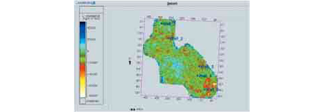
Once the Pseudo Gamma Ray volume has been calculated, it can be interpreted like any other seismic volume. In general, sands should be represented as troughs in the seismic data, with thicker and better quality sands corresponding to larger troughs.

Based on this, an appropriate map to make would be an area under the curve or integration of the seismic values corresponding to the zone of interest. High quality sands should be represented by large negative values on the map.

Figure 30 is a map of the mean Pseudo Gamma Ray response over the Paddy interval. Red blobs correspond to large negative values which should in turn correspond to zones of thick high quality Paddy sands. Further work is currently underway to determine the overall quality of the final product.

Alternatively, a more sophisticated method for interpreting the volume would be to use collocated cokriging to create a net pay map using the actual gamma ray logs as hard variables and the Pseudo Gamma Ray volume as a soft variable.

Conclusions

It has been demonstrated that it is possible to estimate a Gamma Ray Log using Velocity and Density Logs in a zone of consolidated Cretaceous sands.

It is also possible to estimate band-limited Gamma Ray Log response from appropriately processed seismic data.

The Pseudo Gamma Ray Seismic can be combined with Gamma Ray Logs to create maps of high quality sand bodies.

Acknowledgements

I would like to thank Winston Karel, Chris Cade, Steve Campbell and Richard Kruger for help with preparing data used for this paper. In addition I would like to also thank Kristy Howe and Richard Spiteri who were co-authors on the original talk which led up to this paper. Finally I would like to thank Olympic Seismic for permission to show the data and BP Canada Energy for permission to publish.