Predicting Mineralogy from Elastic Rock Properties

In contrast to conventional reservoirs, where the measured elastic rock properties are sensitive to changes in facies, porosity and pore fluids, we find that changes in the elastic rock properties of low porosity unconventional plays are driven largely by changes in the relative fractions of the dominant minerals that form the reservoir rock. Interpretation templates, constructed from rock physics models, can be used to predict mineralogy from the measured elastic rock properties at both the log and seismic scales. The work presented here is similar to previously published reservoir characterization studies, the difference being that here we predict mineral fractions rather than lithofacies. Volumes of mineral fractions predicted from seismic prestack AVO inversion data can be used for geological model building and other studies.

Introduction

Previously, it has been observed that it is difficult to precisely relate mineralogy to elastic rock properties. The probability density function (PDF) of a particular group of minerals derived from well log data can span a large range of elastic rock properties. This may lead to the conclusion that a statistical approach for predicting facies, such as Bayesian classification, is the most pragmatic way to interpret this data (e.g. Avseth, 2000).

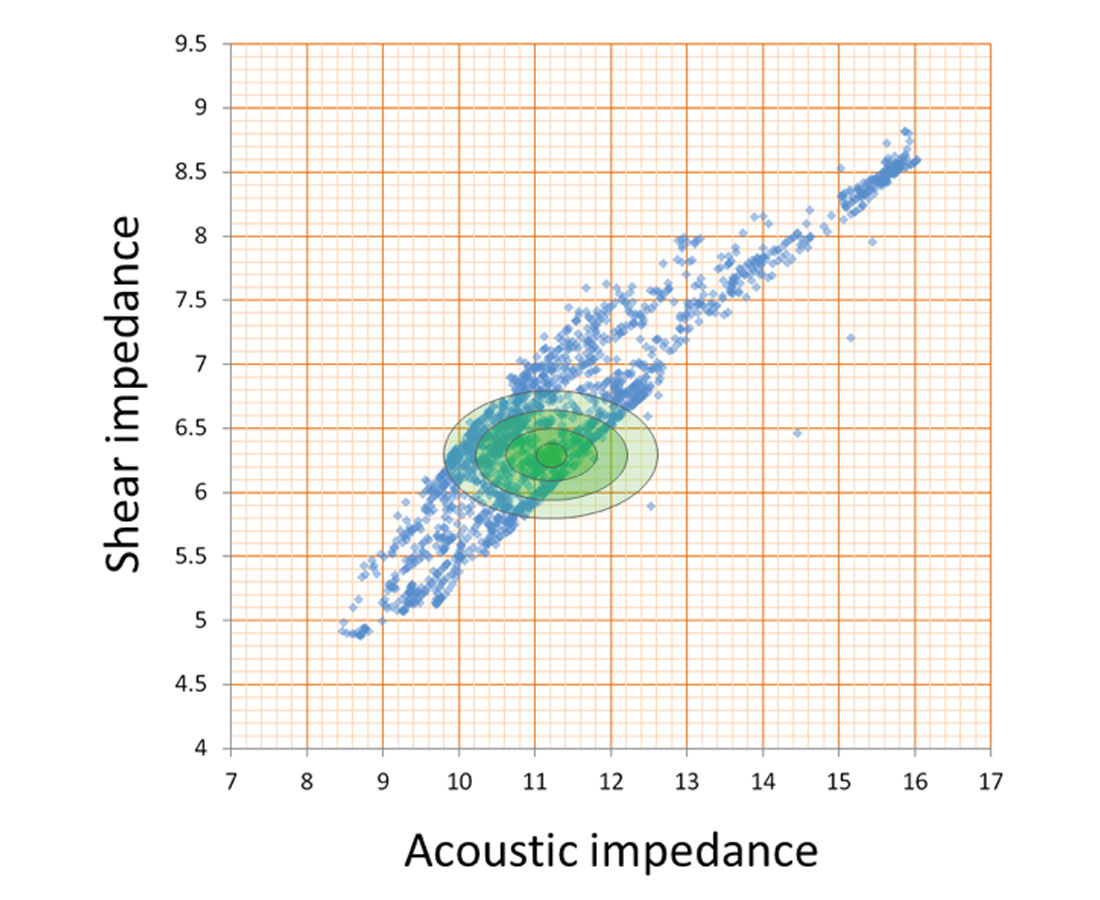
Figure 1 shows the typical scatter of the elastic rock properties (here plotted as acoustic impedance, AI, and shear impedance, SI) measured with our raw well log data for a particular group of minerals. Whilst some of this scatter may be due to differences in the intrinsic mineral properties (from variations in quartz density and velocity caused by variations in the elemental composition of the quartz grains; and from variations in the ratios of the silica minerals grouped together to form the ‘quartz group’), a lot of the scatter is due to other factors including: rock property measurement errors; mineral log errors; variations in other rock properties (water saturation, TOC, porosity, etc.) that also affect the elastic rock properties and are not correlated with mineralogy; resolution differences between rock properties (often lower) and mineral logs (often higher); depth shifts between the mineral log and the sonic and density logs; and changes in these rock properties with changes in effective pressure (depth).

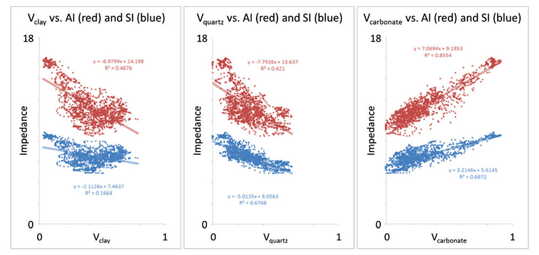
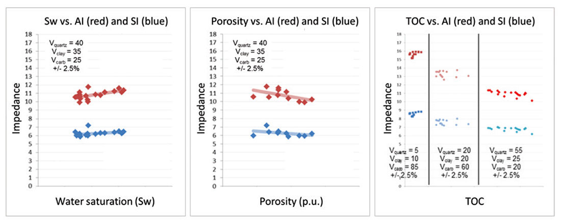
In low porosity unconventional reservoirs, we observe strong correlations between mineralogy and measured elastic rock properties, as shown in Figure 2. The variations of these properties with changes in other rock properties such as porosity, TOC and water saturation are observed to be significantly lower, Figure 3. There are two reasons for this – first, the porosity is low (say < 8%) and relatively constant, so the fluid and porosity effects are small; secondly, there may be correlations between these petrophysical properties and mineralogy which leads to a coupling of these effects with changes in mineralogy.

Predicting mineralogy from measured rock properties using interpretation templates

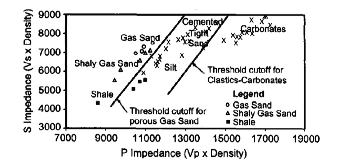
Interpretation templates, constructed from rock physics models, have been used for more than a decade to predict facies (such as sandstone, shale and carbonate) from measured elastic rock properties (e.g. Goodway et al., 1997). When searching for conventional reservoirs, the increased porosity (and the resulting decrease in density) and difference in pore fluid of the reservoir facies compared to the non-reservoir facies separates these facies in elastic rock property space, enabling us to predict reservoir facies and non-reservoir facies from pre-stack AVO inversion data, as shown in Figure 4. In Figure 4 we can also observe that the tight (low porosity) sand does not clearly separate out from the low porosity clay and carbonate facies.

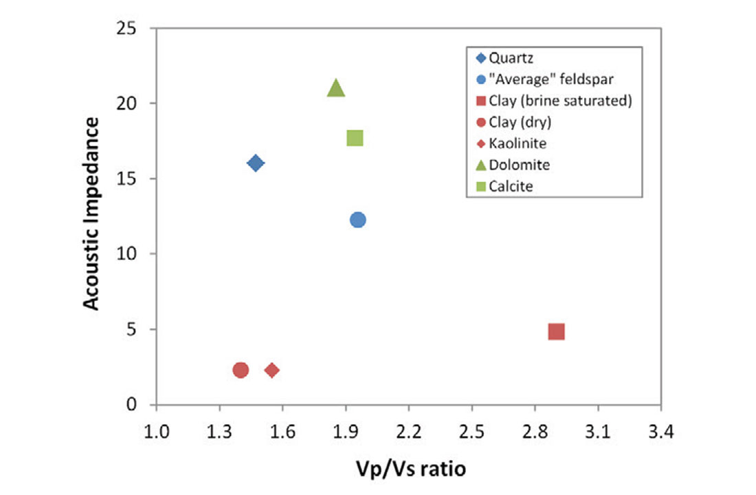
In contrast, zero-porosity pure minerals separate well in elastic rock property space, as shown in Figure 5. We observe that:

1. The acoustic impedance of the carbonates (calcite and dolomite) is greater than that of silicates (quartz and feldspar) and clays. Low porosity carbonate-rich rock will have higher acoustic impedance than low porosity quartz- or clay-rich rock.

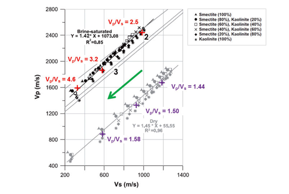
2. The V_p/V_s ratio of quartz, ~1.5, is lower than the V_p/V_s ratio of carbonate, ~1.9. Due to the intercept of the V_p versus V_s trend at the brine velocity when V_s = 0 for brine-saturated clay, the V_p/V_s ratio of brine-saturated clay is variable, and normally higher than that of carbonate, Figure 6. Dry clay has a much lower, roughly constant V_p/V_s ratio. The variations of V_p/V_s for the clay minerals will result in, often small but unavoidable mineral prediction errors from simple rock physics models.

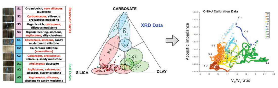
Mineral log data often combine similar minerals together to form mineral ‘groups’. For example, calcite and dolomite are often combined to form ‘carbonate’; quartz, feldspar and mica may be combined to form ‘QFM’; and all the clay minerals (illite, smectite, etc.) are grouped together as ‘clay’. When the ratios of the individual minerals that form these mineral groups are approximately constant, their aggregate properties can separate out in elastic rock property space in a similar manner to that of their constituent minerals, Figure 7.

Rock physics models can be constructed to predict elastic rock properties as a function of mineralogy, porosity, effective pressure, temperature, etc. Often the models are simplified by setting certain rock properties to be constant, such as pressure and temperature. When the range of porosities in our reservoir is small, the models get even simpler (Figure 8), and we find that mineralogy can become the dominant rock property affecting the observed elastic rock properties (here graphed as lambda-rho and mu-rho).

We can construct look-up tables from simple rock physics model-based interpretation templates to predict the relative fractions of the three dominant mineral groups from our measured elastic rock properties for low porosity unconventional reservoirs. When the range of porosities within the reservoir is small, the mineral prediction errors can also be small.

The variable and somewhat similar mineral contents of different low porosity lithofacies (e.g. sands and shales) causes these facies to overlap in elastic rock property space. This creates challenges (and uncertainty) when trying to accurately predicting lithofacies from elastic rock properties.

Mineral predictions from well log data

Well log data from two unconventional plays were used to demonstrate applications of this workflow. Both data sets have Litho Scanner mineral logs, as well as sonic (P- and S-wave) and density logs. Elastic rock properties were calculated from the sonic and density logs. Simple interpretation templates and look-up tables were constructed for both data sets.

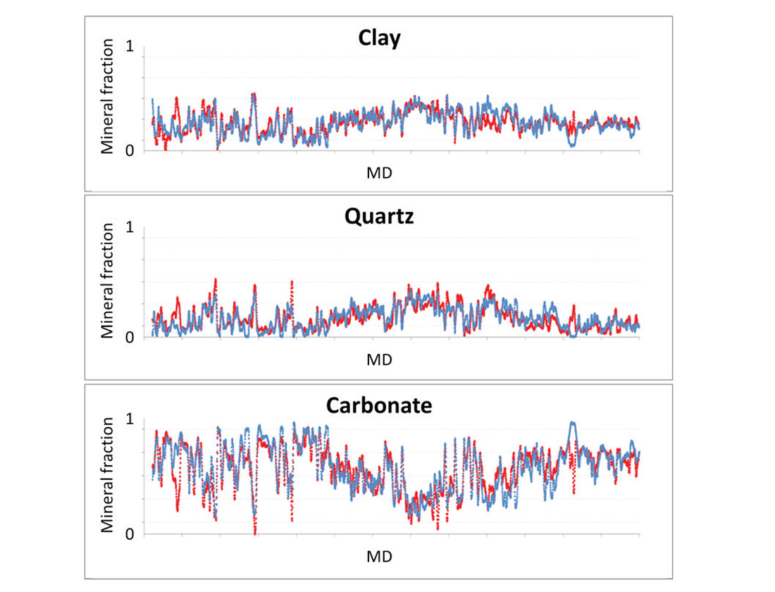
For the first data set, a constant model was sufficient to predict mineralogy from elastic rock property logs with an absolute average difference of ~6 % with the Litho Scanner mineral log data (Figure 9) in areas where the fractions of three dominant mineral groups (clay, QFM and carbonate) summed to 97% or more of the total mineral weight. Tests using blind wells demonstrated that this model could be applied over a large area.

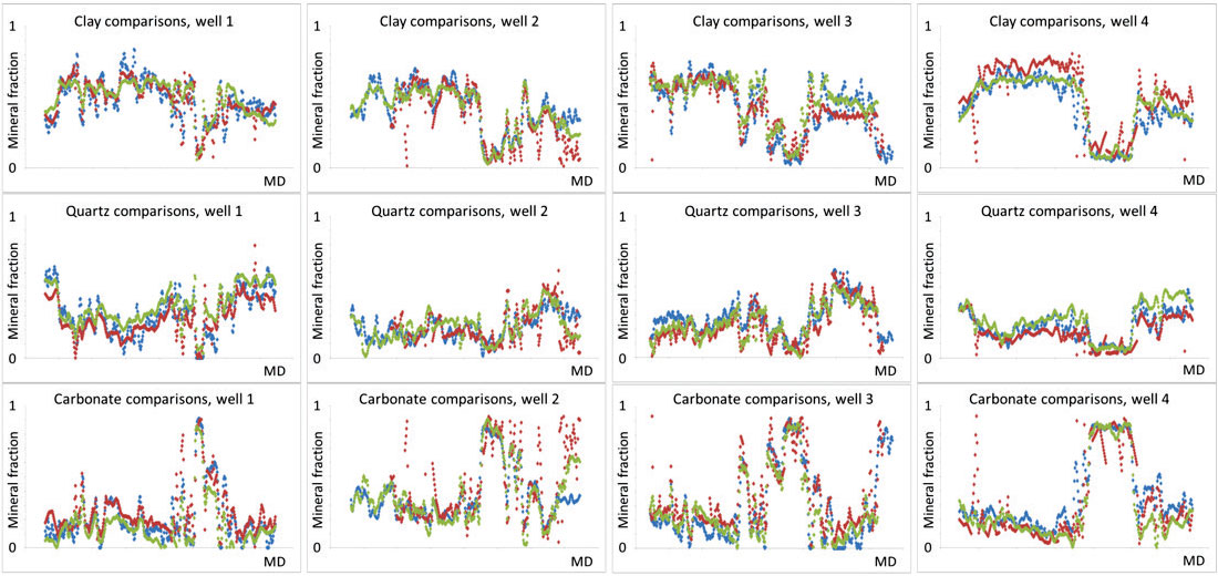
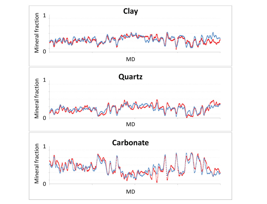
The model used for the second data set, which was built to predict mineralogy over a depth range of ~800m, was adjusted to vary with depth. Again we see an excellent match between the measured and predicted mineralogy (Figures 10 and 11). Areas where the differences between the predictions and the mineral log data are significantly higher than average may identify areas with a mineralogy not modeled (such as salt or basalt), or higher porosity.

Application to seismic data

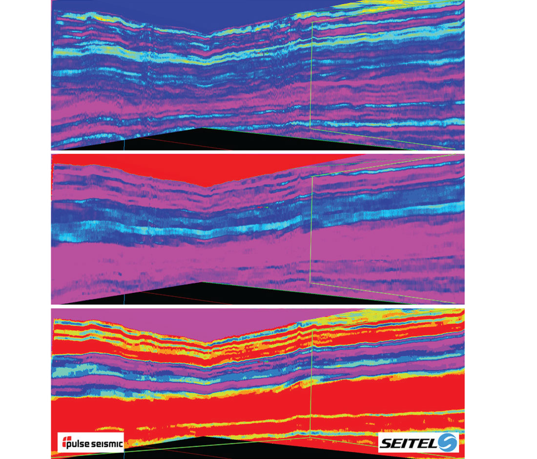
As with facies prediction workflows (e.g. Goodway, 2009), simple rock physics interpretation templates may also be used to predict volumes of mineral fractions from 3D seismic prestack AVO inversion data, Figure 12. Comparing the predicted clay, quartz and carbonate mineral volumes enables us to easily identify different geological formations, which are not so readily interpreted from the prestack AVO inversion data. Scanning through these mineral volumes helps us to understand how the mineral composition of the formations varies temporally and spatially. Comparison with petrophysical data validates these observations.

It is important to note that the quality of the seismic-scale mineral predictions is fully dependent on the quality of the elastic rock properties that come out of prestack AVO inversion. Seismic processing errors, errors in the low frequency model, and inversion errors map directly into mineral prediction errors. We observe, for example, that that the mineral predictions lose continuity in noisy data areas in exactly the same way as traditional amplitude-based interpretations.

Conclusions

Using simple rock physics models, we can predict mineralogy from measured elastic rock properties for the characterization of low porosity unconventional reservoirs. The differences between the predicted mineral fractions and mineral log data can be easily quantified. This gives us confidence that we can use these predictions for geological mapping and other studies.

Acknowledgements

We are most grateful to Shell for permission to publish the results of this work. Many of our colleagues at Shell gave us valuable feedback during the development of the workflow, and also kindly provided access to their well and seismic data. Permission to publish derivatives of the licenced seismic data courtesy of Pulse Canada and Seitel Canada Ltd.