Practical applications of P-wave AVO for unconventional gas Resource Plays – I: Seismic petrophysics

Introduction

For the past few years natural gas exploration in North America has focused on the huge resource potential of unconventional reservoirs such as coalbed methane (CBM), tight gas sands and shales. These gas accumulations, termed Resource Plays at EnCana, are low permeability-porosity reservoirs, with gas stored in natural fractures or cleats, within the matrix porosity and adsorbed onto the surfaces of kerogen. As these reservoirs exist throughout the Rocky Mountains, Texas, Oklahoma and the Appalachian Basin, most of the industry drilling activity has been in the US. In Canada similar Resource Plays within the Western Canadian Sedimentary Basin (WCSB) are in the initial stages of exploitation.

Due to the low permeability of these Resource Plays, hydraulic fracture stimulation is required to achieve gas production and effective stimulation requires either the connection to existing natural fractures or the presence of geomechanical brittleness capable of supporting extensive induced fractures. However, not all tight gas reservoirs are created equal despite their thick, continuous nature and any given well can be uneconomical to drill. Variation between wells in stabilized gas rates and economic ultimate recovery (EUR) can only be explained by the heterogeneity typically encountered in these Resource Plays. Natural fractures or fracability, porosity and gas saturation are important criteria in identifying the correct well location. Consequently the use of 3D seismic, AVO and AVO variation with azimuth (AVAZ) to detect anisotropy due to fractures, stress or over- pressure are essential to the development success of such plays.

Part 1 of this paper describes the rock mechanics, petrophysics and conventional isotropic AVO that can be applied to map Resource Play potential and predict optimal drilling locations. Part 2, deals with some fundamental ambiguities involved in azimuthal AVO methods to correctly detect the orientation and degree of anisotropy. Understanding the limitations of these ambiguities will be illustrated by 3D data studies from the WCSB and puts constraints on the ability of the technology to establish the presence and recovery of tight gas.

Mechanical characteristics of tight gas reservoirs from a petrophysical seismic perspective

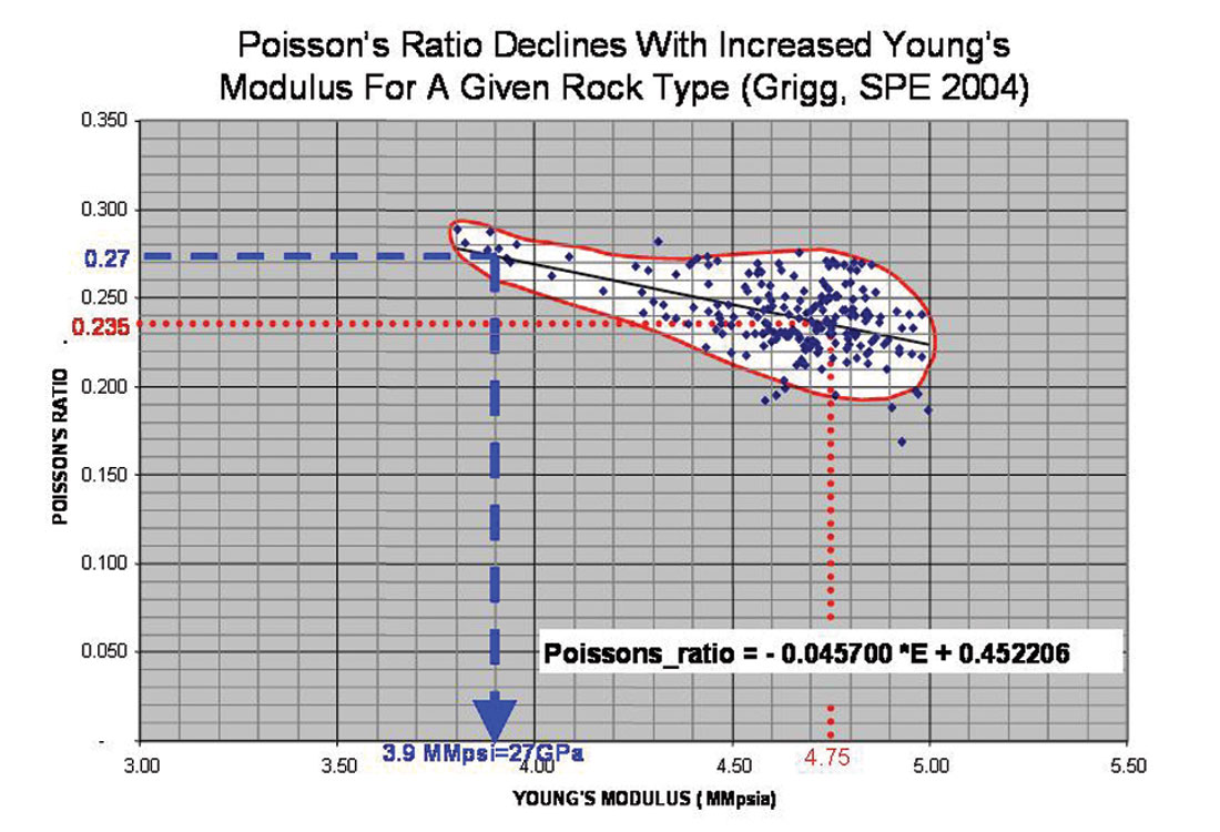
As tight gas Resource Plays are low porosity and generally fully gas charged, the application of AVO methods is simplified to primarily extracting lithologic and mechanical properties from seismic data. By contrast, AVO for conventional plays must account for the confusing mix of lithology, fluid saturation, compaction and over- pressure. An example of this analysis is shown here for the gas shale case, but the methods are equally applicable to CBM or gas sands. Commercial production of gas shale has not yet been achieved in Canada, but is well established in plays such as the Barnett shale of Texas. Consequently the mechanical characteristics of the Barnett shale are used as an analogue to help guide AVO techniques in identifying the resource potential of similar shales. Engineering literature focuses on identifying optimum Barnett shale mechanical properties of Young’s modulus (E) and Poisson’s ratio (ν) as shown in figure 1 (Grigg, SPE 2004). In order to better understand the significance of E and ν, these parameters are converted to the simpler and more intuitive Lamé parameters of incompressibility Lambda (λ) and rigidity Mu (μ) (Goodway et al 1997, 2001) through the following relationships:

From above E and ν can be related as:

An initial observation is that the inverse linear relation between increasing E to decreasing ν shown for the Barnett shale in figure 1, is simply the result of an increase in rigidity μ.

Relating both λ and μ to E and ν, so as to compare mechanical properties on equivalent log cross-plots, is not so simple as E has a non-linear relationship to the ratio of Mu to Lambda (μ/λ).

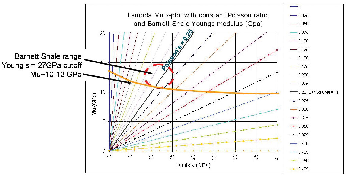
However by using the relationship above a graph can be constructed showing Young’s modulus vs. Lambda with curves of constant Mu and lines of constant Poisson’s Ratio (figure 2).

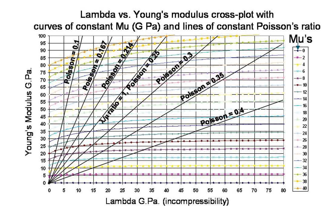
The Barnett shale ranges shown in figure 1 above, of Young’s modulus (4-5 MMpsi) and Poisson’s ratio (0.2-0.3), give cutoff values for high μ rigidity > 10 G.Pa and Lambda/Mu ratios around 1:1 as shown in figure 3. This template can now be used to guide the petrophysics and seismic AVO expectation to identify similar gas shales.

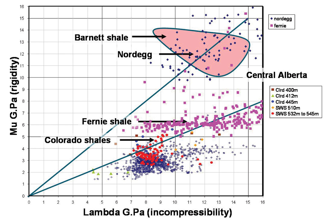
Based on this template, log data from various shale and sand lithologies within the WCSB are compared to the Barnett shale as shown in figure 4. From the four zones shown, Nordegg, Fernie, Colorado (Clrd) and 2nd White Specks (SWS), only the Nordegg appears to have similar λ, μ values to the Barnett shale. By contrast the Colorado/SWS group’s μ rigidity values of at most 5-6 G.Pa (light blue, red, orange points) are lower by a factor of two from the productive Barnett gas shale but have a similar range of λ values.

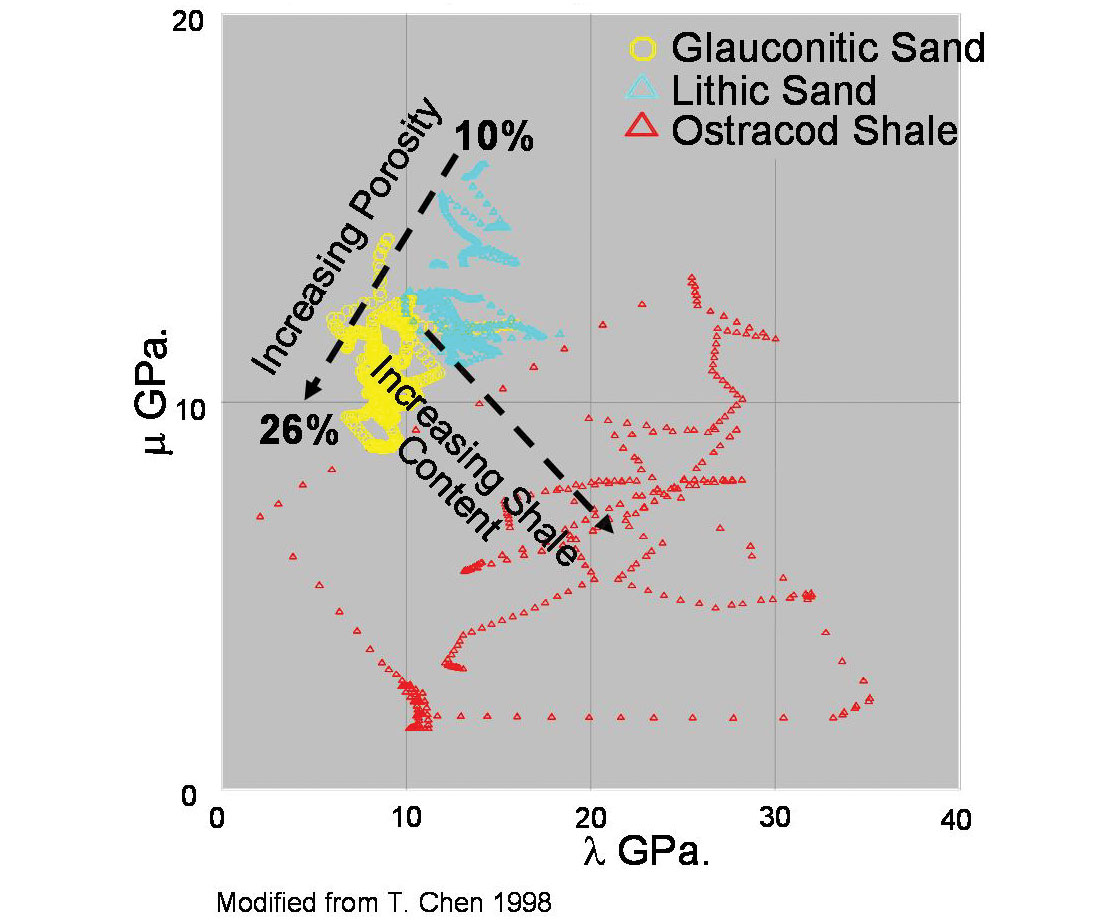
Despite this, the conclusion of requiring as high a Mu or MuRho (μ ρ) parameter as possible to support natural or induced fractures is used in the 3D seismic AVO/LMR (Lambda, Mu, Rho) analysis and inversion in the next section. Before leaving the Barnett shale comparison, interpretation of the λ, μ cross-plots suggest the best zones appear to occupy areas more commonly associated with lithic gas sands, shown by the blue points in the conventional log based LMR template in figure 5 (Goodway et al 2001).

This observation is not surprising considering that the reason for the Barnett shale’s ability to support natural or induced fractures (fracablity) is due to its unusually high quartz content for a shale. From an engineering perspective a rock’s fracablity is governed by the closure stress equation that is a function of E and ν as shown below, giving rise to the emphasis on these properties for the Barnett shale.

Where σ_xx = minimum horizontal (closure) stress, σ_zz = overburden stress, e_xx,e_yy,e_zz = strains in x,y and z

P_P = pore pressure, B_V and B_H = vertical and horizontal poroelastic constant.

In a similar manner to that used above to convert E and ν to λ and μ, the closure stress equation can be written as:

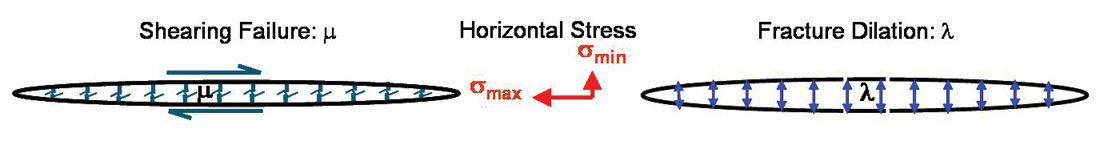
Now the most fracable zones occupying relatively low λ’s and high μ’s in the cross-plots above, can be understood as also having the lowest closure stress, governed by the λ/(λ+2μ) ratio term in equation (2). The influence of Lambda and Mu on horizontal closure stress is captured in diagram A, where rigidity Mu determines the rock’s resistance to transverse or shear failure and Lambda is the rock’s resistance to fracture dilation that in turn relates to pore pressure.

Diagram A

Petrophysically the Barnett shale is a black, siliceous source rock with 4-8% organic carbon content (TOC), 20-40% illite clay, and no free water. Gas occurs as free gas in the matrix, free gas in fractures, or absorbed gas. In order to compare these additional Barnett shale characteristics, a detailed petrophysical and core analysis was run on Colorado shales from Central Alberta, to relate high TOC (kerogen) or adsorbed gas potential to the mechanical or elastic properties of high MuRho rigidity established above. The results, shown in the log tracks in figure 6, identify a series of zones with high TOC (circled red dots) and high μ ρ, low λ/μ ratios (boxes marked on rightmost LMR, S-impedance and density tracks). The most prospective zones are seen just above the top of the Colorado B (Clrd B) at 445m and in the lower half of the 2nd White Specks (SWSpk) at 510m and between 530m and 550m.

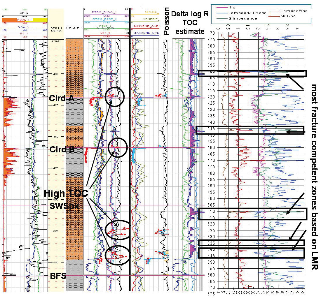
The red and light blue dots in the middle tracks for core vs. log estimates of high TOC zones, show a good correlation. Furthermore all the boxed zones identified as having the most comparable mechanical properties to the Barnett shale, also have a strong correlation to the “delta log R” estimate of TOC shown by the purple/pink flags just to the left of the boxed zones.

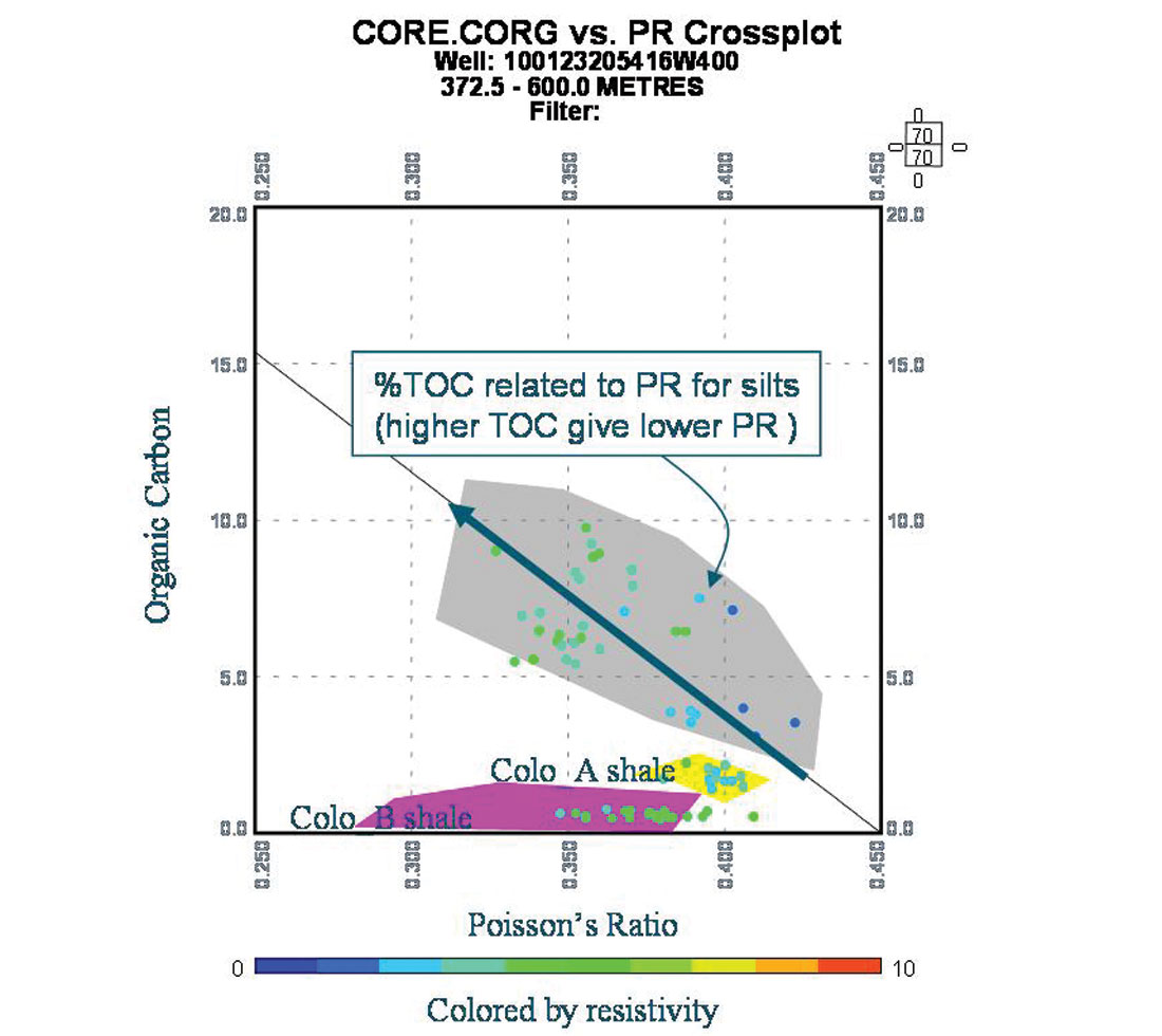
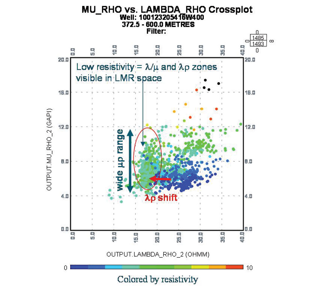
Cross-plots in figures 7a, 7b, below, show a further relationship between resistivity, TOC and mechanical or elastic properties of Poisson’s ratio and LMR. Correlation of high TOC with low Poisson ratio in cross-plot 7a, is probably a result of a gas effect from high TOC zones that would lower Poisson’s ratio. This is more evident on the LMR cross-plot in 7b, where zones of higher resistivity (blue to green overlay) appear as a shift to lower λρ values from increased gas saturation. Interestingly, this high resistivity low λρ cloud has a wide μρ range, where the most fracture prone points have the highest values based on the Barnett shale’s LMR analysis above.

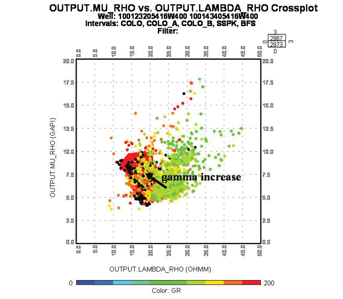
In figure 7c, however, there is an unusual correlation of high gamma values with increasing μρ and decreasing λρ i.e. in the direction of increasing quartz content. This seemingly inconsistent LMR trend is consistent with the high resistivity to low λρ trend in figure 7b, as a high resisitvity response from a gas effect can be related to high gamma readings in a shale from these organic rich zones.

AVO for mechanical rock properties

Following the results of the log and core analysis, AVO inversion was run on a 3D dataset to extract mechanical or elastic attributes described in the previous section.

Three quite different methods, will be compared for their accuracy in extracting AVO attributes for mechanical rock properties. All three are based on the P-wave angle dependent reflectivity formulation given by Aki and Richards (1980), as shown in the equation (a) below. This equation is in terms of fractional changes in velocities Vp, Vs and density rho, that are equivalent to reflectivity contrasts across an interface and is accurate even beyond the critical angle for small reflectivity contrasts as shown recently by Downton et al (2005).

where

From this starting point the three methods are based on further two term approximations used to obtain robust estimates of the following elastic parameters:

1. P-wave and shear wave reflectivities Rp(0), Rs(0) which can be inverted into λρ and μρ
2. Rp(0) and pseudo-Poisson reflectivity that might be used directly in hydraulic fracture stimulation
3. P-wave velocity reflectivity ΔVp/Vp and Mu rigidity reflectivity Δμ/μ.

Method 1 “Gidlow/Fatti”: This method estimates Rp(0) or fractional P-impedance change ΔIp/Ip and Rs(0) or fractional Simpedance change ΔIs/Is as “seismic traces” through “weighted stacking” of CMP gather data (Gidlow et al 1992, Fatti et al 1994). The equation used in this extraction is an algebraic rearrangement of the Aki & Richards equation above given as;

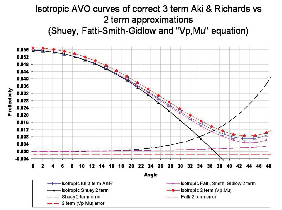
Equation (b) known as the “Geogain Equation” from Gidlow et al, is solved using least squares or the L1 norm to estimate Rp(0) and Rs(0) from the first two terms, by assuming that the third term cancels at small angles and for small density contrasts. If the density contrast is not small then this third “error” term can be significant at large angles. More importantly, given the sensitivity of azimuthal AVO gradient requirements to be considered in the second part of this paper, these limitations may lead to predictions of the wrong gradient for varying rock properties by being dependent on both angle and Vp/Vs ratio. However this limitation is mitigated when applied to Resource Plays, as density contrasts are generally small in these tight formations. So in the case study considered here, the method can be practically applied to fairly large angles (see model AVO curve comparisons in figure 8) given that Δρ/ρ is small and also not nearly as significant as ΔVp/Vp as seen in Gardner’s (1974) relationship: Δρ/ρ ≈ (ΔVp/Vp)/4.

Consequently restricting the angle range due to the ignored error term and thereby reducing the curvature separability of the first two sine and tangent terms, is not advised, as this will lead to less robust and less independent estimates of the key elastic reflectivities; ΔIp/Ip and ΔIs/Is.

Method 2 “Shuey”: This method is based on a two term approximation (Shuey 1984) with a significantly more complex formulation than the Gidlow/Fatti equation (b) above and is just reproduced here for comparison.

where σ = Poisson's ratio and

The Shuey two term approximation for equation (c) is to drop the third term in (ΔVp/Vp) thereby severely restricting the usable angles to ranges less than 20° or 30°, because ignoring a term in (ΔVp/Vp) is much worse than ignoring a Δρ/ρ term in the Gidlow, Fatti et al equation (a). AVAZ methods (covered in part two of this paper) that rely on gradient curvature will give ambiguous and even meaningless results by using this approximation.

Method 3 “Wang/Goodway”: This method (termed “Vp, Mu” in figure 8) shows a less common formulation for linearized P-wave AVO and is obtained by simply substituting the following relationships into the original Aki & Richards equation:

to give

The two term approximation for this equation (d) (Wang 1999, Goodway 2001), is to drop the small zero offset term Δρ/2ρ (again from Gardner’s relationship Δρ/2ρ ≈ (ΔVp/Vp)/8). This results in an error that is independent of angle unlike the Gidlow, Fatti et al or Shuey two term approximations and allows a more accurate curvature fit to the exact three term Aki & Richards AVO curve at large angles. However there is a “bulk” Δρ/2ρ scalar shift at all angles. Because of the accurate gradient predictions this is the best method for AVAZ and forms the basis for Ruger’s 1997 equation, to be covered in part two.

These three two term approximations (equations b, c and d) are compared in figure 8, for accuracy in matching the three term Aki and Richards equation, using log values from zones identified in the previous section.

Notice that the Shuey two term approximation has significant error past 28° and gives rise to the commonly accepted angle restriction that creates significant ambiguities for common methods using AVAZ to estimate anisotropy. By contrast the other two term approximations allow for the extraction of elastic and rock property information contained in the AVO curvature term for angles well beyond 30° and the importance of this for AVAZ will become apparent in part two.

The AVO model curves in figure 8, show a high impedance, high μρ type 1 AVO event for log values taken from the most prospective zones in the Colorado B at 445m and in the 2nd White Specks between 510m and 550m.

The 3D survey used in this AVO- AVAZ study was optimally acquired with a wide-azimuth, high density far- offset MegaBin acquisition (Goodway, Ragan and Li 1996), thus facilitating an exceptionally good analysis of offset and azimuth AVO variations. An actual 3D azimuth-offset gather in figure 9, shows a good AVO type 1 match for zones of high MuRho rigidity contrast, at both the top of the Colorado B and within the 2nd White Specks, that might support potential natural or induced fractures as predicted by log analysis in the previous section.

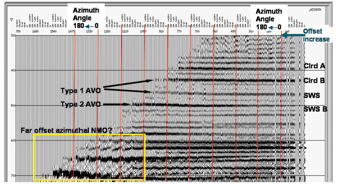
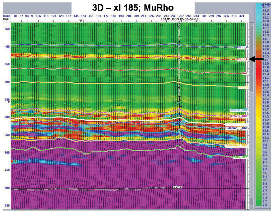
Figure 10, shows a MuRho section from an LMR inversion of the 3D based on the “Geogain Equation” from Gidlow et al (method 1, above). The black arrow marks a shallow, high MuRho zone ( red, yellow colours) identified as being at the top of the Colorado B (red horizon Clrd B), that coincides with the predictions from the log analysis for the well that is located on this line as shown.

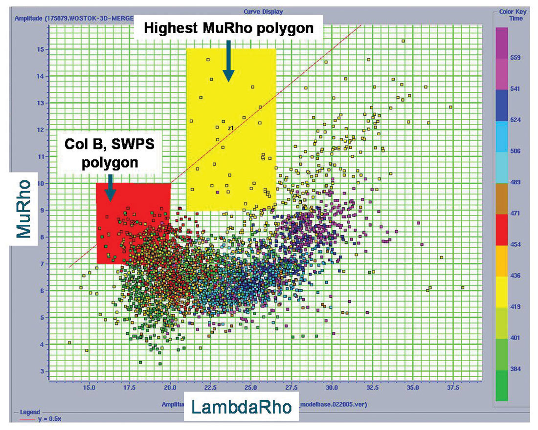
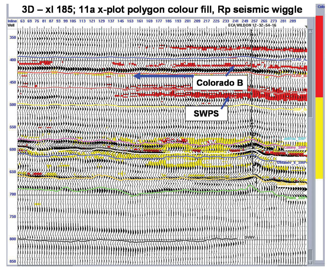
The LMR cross-plot and resulting polygon section shown in figures 11 a and b, are of inversion results for the same 3D crossline shown in figure 10.

In this interpretation the highest MuRho and lowest LambdaRho zones are clearly isolated at the top Colorado B (Clrd B ~ 425 ms) and mid to base 2nd White Specks (SWP-SWP B 450-500 ms) by the red LMR cross-plot polygon. The Colorado B zone even has a few very high MuRho values (blue arrow in figure 11b highlighting yellow cross-plot polygon points) that approach those of the Barnett shale analogue.

The second part of this paper to follow in April 2006, will investigate and describe the AVAZ issues involved in analyzing the same 3D dataset. The isotropic AVO/LMR attributes shown above will be combined with AVAZ attributes representing fracture density and orientation to select areas with the best probability of high fracture intensity and good gas charge.

Acknowledgements

Dave Gray, Dragana Todorovic-Marinic and Jay Gunderson (Veritas DGC)