New developments in audio-magnetotelluric exploration: Case study from Darnley Bay area, N.W.T

Darnley Bay occurs within the Amundsen Gulf and is located within the Inuvialuit settlement region of the Western Canadian Arctic. It is home to one of the largest gravity anomalies in the world. With a diameter of approximately 60 km and an amplitude exceeding 130 mGal, the source of the gravity anomaly is thought to be a large igneous intrusion. However, the depth and orientation of the postulated intrusive body remain a point of debate.

In an effort to help answer these questions, a transient magnetotelluric survey was conducted over the western half of the Darnley Bay gravity anomaly. A deep, weakly resistive feature was revealed, which if corresponding to the postulated intrusive body, indicates a depth in the range of 2.5 to 3.2 km. Although poorly resolved, the deep resistive body appears to be upthrust beneath our survey line, with evidence of fault structure bracketing each side of the proposed upthrust block.

Introduction

Magnetotellurics (MT) makes use of naturally occurring fluctuations in the earth’s magnetic field which, by induction, cause electrical currents to flow within the earth, the size of which are determined by local earth resistivity. Information as a function of depth is obtained through making measurements across a broad frequency range, penetration depth increasing as frequency decreases. When measurements are made in the frequency range above 1 Hz, the modifier audio is added, or simply AMT.

Compared to controlled source methods, AMT is logistically simpler, requiring less field personnel and equipment, and is capable of cost effectively exploring to great depths. However, the natural signals are not under our control and suffer from frequency ranges with little or no signal. Most notably, the AMT “dead-band” between approximately 1 kHz and 4 kHz, but also a signal low in the vicinity of 1 Hz where the transition to magnetospheric energy sources occurs.

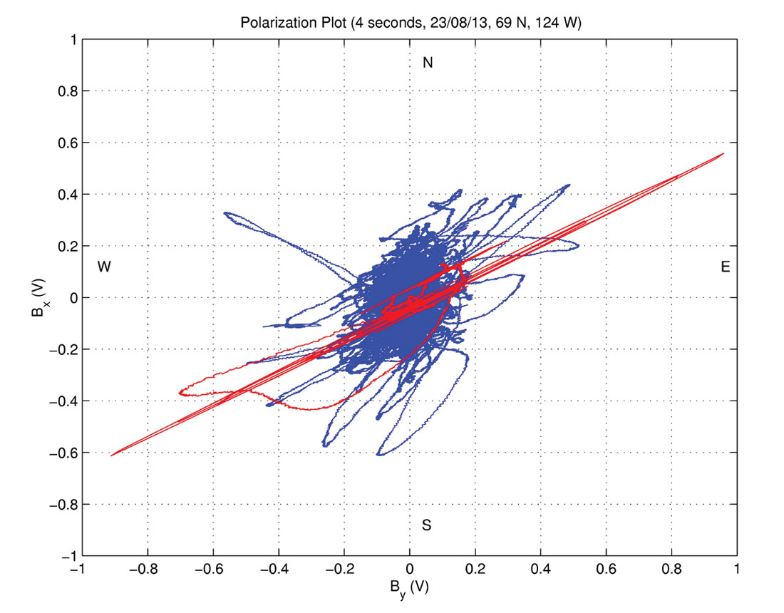
The natural electromagnetic source field in the frequency range above 1 Hz is predominantly due to lightning discharges and can be divided into two main components. A transient component due to individual lightning discharges (sferics) and a low-level quasi-continuous component due to the random, incoherent sum of near global activity (Tzanis and Beamish, 1987). The two components have completely different polarization characteristics; the transient component being linearly polarized (Figure 1, in red) while the low level continuing component typically elliptically, or ideally (for conventional processing), circularly polarized (Figure 1, the blue centre of mass). Note that the direction of sferic propagation is perpendicular to the direction of magnetic field oscillation.

However, global waveguide attenuation is such that the continuing component is most significantly present in two relatively narrow frequency ranges. Namely, between 8 Hz and 200 Hz, and even less so from 7 kHz to 15 kHz. These are the frequency bands in the ELF/VLF¹ range where global waveguide attenuation is lowest.

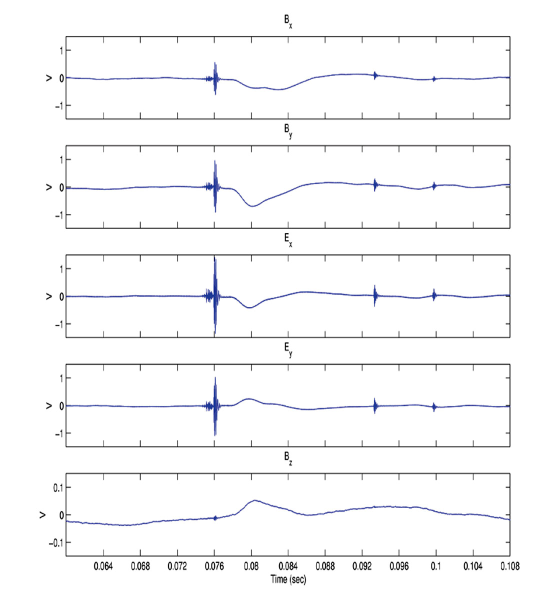
order to increase signal-to-noise ratio (SNR) and enhance data quality, especially outside of the continuing windows, our transient approach to AMT centers around the time localized recording of individual transient events (sferics). This is not new and has been done by many others, including Hoover et al. (1976), Tzanis and Beamish (1987), Kosteniuk and Paulson (1988), Vozoff (1991, describing instrumentation built at McQuarie University in the 1980’s), Garner and Thiel (1999). Shown in Figure 2 is the time series corresponding to the sferic in Figure 1. Due to dispersion, VLF and ELF wavelets arrive separated in time with the amount of separation indicating distance to the source (Hepburn and Pierce, 1953). In this case, a separation of approximately 4.4 ms indicates a distance to the source of 7600 km. Note that without measurement of the vertical electric field, we don’t know if this event came from the SE (Central America) or over the polar ice cap from the NW (Mongolia). The interested reader is referred to www.empulse.ca for examples of vertical electric field measurements with sferics.

However, while many others have adopted a transient recording method, all except for Kosteniuk and Paulson (1988) used standard AMT processing techniques designed more so for elliptically or circularly polarized data. It has been shown that the polarization diversity of linearly polarized events causes a bias in Remote-reference results additional to that caused by finite SNR and sample size (Goldak and Goldak, 2001).

Therefore, we extended the Polarization Stacking algorithm of Kosteniuk and Paulson (1988) to be adaptive to the constantly changing bearing and amplitude characteristics of linearly polarized, transient data (Goldak and Goldak, 2001). A key feature of our Adaptive Polarization Stacking (APS) algorithm is that we are able to enhance SNR, at least to an extent, through a time domain stacking of the transient waveforms. This results in essentially unbiased estimates of earth response curves, even with narrow angle sources.

The main benefit of our transient approach to AMT is enhanced data quality and bandwidth, especially the tipper, but also the high frequency impedance. The interested reader is referred to Goldak and Kosteniuk (2012) for a more complete comparison of transient and conventional approaches to AMT and Goldak and Goldak (2001) for a theoretical analysis of the bias performance of our APS algorithm. This information is also available on our website, www.empulse.ca.

The impedance tensor Z(ω) and magnetic field tipper T(ω) are the fundamental quantities of interest in a magnetotelluric survey. The impedance tensor is the transfer function between vector components of electric and magnetic fields, as defined in equation (1) in the frequency domain.

The magnetic field tipper is defined in equation (2). The tipper relates vertical and horizontal components of the magnetic field alone and is sensitive to lateral changes in resistivity, especially vertically oriented contacts and long strike length features as these are excellent current channelers. Note that in a purely layered earth, the tipper is zero.

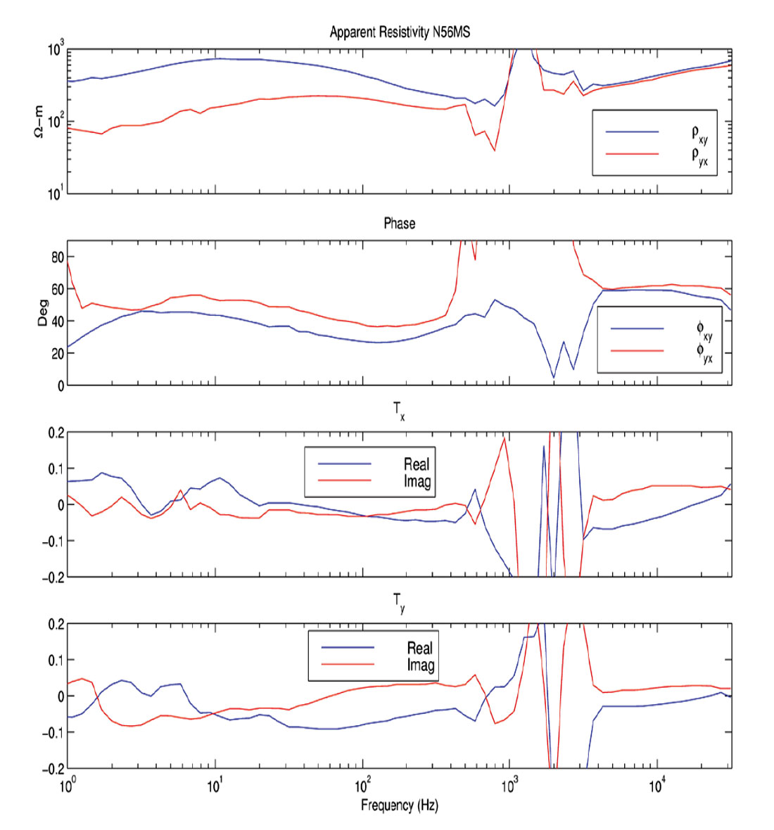
The apparent resistivity is essentially the magnitude squared of the impedance and the phase is simply the argument of the impedance. Shown in Figure 3 are the raw xy, yx and tipper curves for station 56. Note the increased scatter in the “dead-band” from approximately 1 kHz to 4 kHz in all cases. Due to local ground conditions, the vertical coil was not buried very effectively ², therefore, tipper data quality below 20 Hz was in general quite low due to motion noise.

Within the study area, Phanerozoic cover is on the order of 1 km thick, gently east dipping and consisting of tens of metres of glacially derived sediments overlying mostly carbonates, the thickest unit of which are silicified carbonates of the Ronning Group (Reford, 2012).

At approximately 1.2 km depth, relatively conductive mudstones of Proterozoic age, known as the Shaler group, extend downward for yet another 1 km approximately (Reford, 2012). Below the Shaler group typically lie carbonates of the Dismal Lakes and sandstones of the Hornby Bay Groups (Cook and Maclean, 2004).

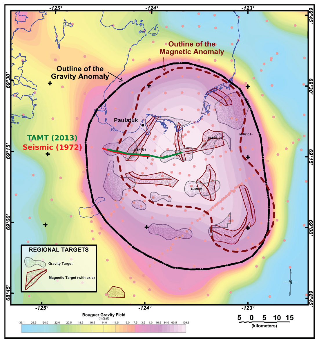
Although the magnetic component of the anomaly was first detected in 1954 by pilots noticing anomalous compass behaviour in the area of Darnley Bay, it wasn’t until 1969 that the Geological Survey of Canada performed a large scale gravity survey and mapped the gravity signature of the entire anomaly (Figure 4, modified after Reford, 2012). In 1972, Sigma Explorations Ltd. collected a 2D reflection seismic profile for Arjay Kirker Resources over the western half of the anomaly (Figure 4). Although the upper 0.4 seconds of data were not useable, several prominent East dipping reflectors were noted along with a vertical offset near the western edge of the magnetic anomaly, interpreted to be due to a fault. Note that the current transient audio magnetotelluric survey (TAMT) survey for the most part, follows the same survey line as the 1972 seismic survey (Figure 4).

Vye (1972) interpreted a prominent reflector at 0.4 to 0.5 seconds as the top of Cambrian and a stronger series of East dipping reflectors at approximately 1.5 seconds as the top of the intrusive body. Although no sonic or density logs were (or are) available in the immediate area, Vye (1972) indicates a depth to the intrusive body of 3048 m to 3354 m.

Analysis of the gravity data by Stacey (1971) indicates that a truncated cone model fits the gravity data quite well, whether the cone expands or narrows with increasing depth. Taking into account airborne magnetic data as well, Stacey (1971) concludes that the most likely model is a truncated cone which expands as depth increases, with the top of the intrusive body between 1 and 5.5 km depth.

However, later analysis of the gravity data indicates that a steep sided intrusive body as deep as 7 km will also fit the gravity data (Jefferson, 1994) and that the seismic reflectors previously interpreted as the top of the intrusion could alternatively represent deformed sediments of the Dismal Lakes group (Cook and Maclean, 2004).

Drillhole DBR-001 (Figure 4) was collared in April, 2000 in an effort to intersect the presumed intrusive body. Due to difficulties encountered while drilling, the hole was terminated at a depth of 1812 metres and did not intersect an igneous intrusion. However, DBR-001 revealed the thickness of the Phanerozoic at 1167.5 m, the hole was terminated within Proterozoic sediments of the Shaler Group (Reford, 2012).

Survey Parameters

TAMT survey coverage is shown in Figure 4, a total of seventy-four stations were collected with a spacing of 500 m, data bandwidth is 1 Hz to 31.5 kHz. Typical recording time was 30 minutes with full 3 component recording of Hx, Hy, and Hz with low noise field feedback induction coil magnetometers (of our own design and construction). The electric field was measured with lead-lead-chloride porous pot electrodes spaced 50 m apart. Analog signals were amplified and filtered prior to 16 bit digitization with a sample rate of 125 kHz. Upon triggering, a total of 524,288 samples were recorded with 10,000 pre-trigger samples retained. In accord with geomagnetic convention, a co-ordinate system with positive x to the North, positive y to the East and positive z down was used.

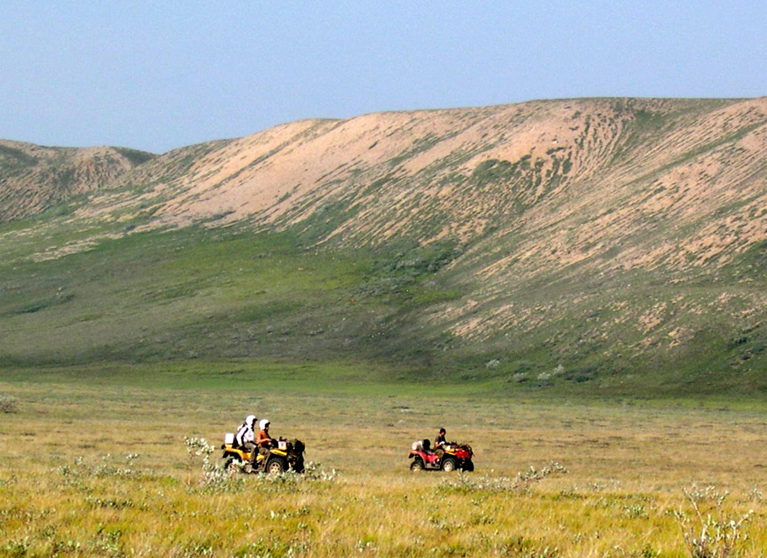
Two survey crews were based in Paulatuk and the survey line was accessed daily with all-terrain vehicles (Figure 5). Due to tussocks and many low lying wet areas, we were able to average only 10 km/hr. Therefore, a distance of 20 km from base was about as far as we could venture as even this required more than 4 hrs of travel time round trip. As a result, survey production per crew was rather low. However, with the use of two crews, we were able to average 9 stations per day.

Survey Results

Static shift is a major issue for this data-set; caused by charge accumulation at the boundaries of near surface 3D inhomogeneities, the electric field can be shifted up or down by an unknown frequency independent factor. This results in vertical displacements of the apparent resistivity curves (and impedance).

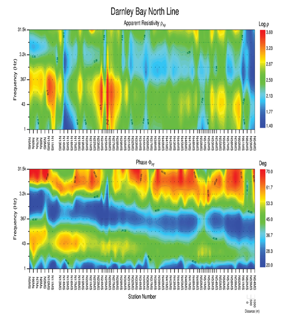
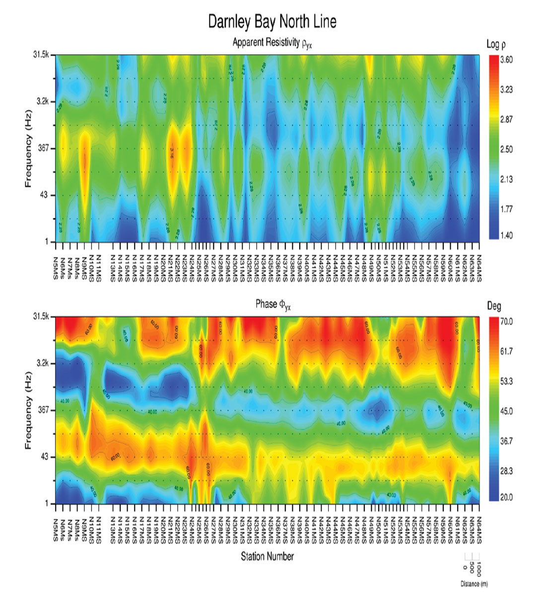
The edited xy apparent resistivity and phase is shown in Figure 6 while the yx apparent resistivity and phase is shown in Figure 7. Note that in both cases, the phase is by comparison very smooth and self-consistent as compared to the apparent resistivity. The phase low (in blue) at approximately 500 Hz in Figure 6 is due to silicified carbonates of the Ronning Group, which show a clear dip to the East. The phase high (in red) at lower frequency in Figure 7 is due to conductive mudstones of the Shaler group.

It is a well known feature of MT data that the phase, depending only on the argument of the impedance, is not affected by statics. Similarly, the magnetic field tipper is also (mostly) not affected by statics. However, any tipper anomalies that did occur were fairly small (less than 20 percent), so a 3D tipper inversion by itself did not yield very useful results. Since the 3D inversion code WSINV3DMT (Siripunvaraporn, 2005) does not model statics explicitly, it was essential to static shift correct the impedance data prior to 3D inversion.

Therefore, 2D phase inversions were conducted whereby the 2D OCCAM code (deGroot-Hedlin and Constable, 1990) was allowed to fit the phase to within our prescribed error bars while those on the (static shifted) apparent resistivity were made very large. In this fashion, we were able to obtain a modeled resistivity that is consistent with our measured phase (at least in a 2D sense). Static shift factors were then obtained as the ratio of the modeled resistivity divided by the measured resistivity (in log space). The impedance tensor elements were then static shift corrected by ensuring that the corrected impedance tensor reproduces the static shift corrected apparent resistivity.

To invert the impedance and tipper data in 3D, a parallel version of WSINV3DMT was used with a model comprising 33 cells N-S, 137 cells E-W and 48 cells vertically. Within the area of interest, a cell size of 250 m was used, which then progressively increased as we transitioned into background. Twenty-three frequencies from 1 Hz to 31.5 kHz were used for data input, only 3 iterations were required to fit Zxy, Zyx, Tx, Ty to an RMS misfit of 0.997 ³ . This required 10.5 hrs to complete on our 36 core, 64 bit Linux cluster. For projects with less than 400 stations, 3D inversion with our small cluster has become quite routine and very effective, fitting the impedance and tipper data in the most general fashion, i.e., with a minimum of assumptions.

Shown in Figure 8 is a vertical slice out of the 3D inversion cube, directly down the survey line, with reflection seismic overlain and lithologic contacts from drillhole DBR-001 indicated ⁴. A constant vertical scaling of the seismic data to depth was accomplished by aligning the 0.4 sec reflector with the top of the Cambrian horizon, as per Vye (1972). Although very approximate, horizons scaled as such appear to overlay the 3D TAMT inversion quite respectably.

Working from shallow to deep, there is an overall gradual East dip seen with near surface glacially derived sediments (mostly in green) increasing in thickness from less than 50 m at the West end of line to approximately 200 m at the East end of line. This agrees with refraction studies carried out by Vye (1972) who indicated a thickening of Cretaceous sediments to over 700 ft at the East end of the seismic line.

Below approximately 100 m (West end) to 200 m (East end) a resistive layer (in red) is seen to approximately 1 km depth (Figure 8). This is mostly due to silicified carbonates of the Ronning Group/Franklin Mountain formation, seen from 377 m to 964.5 m in DBR-001. Although another layer of carbonates, the Hume formation, is noted from 136 m to 365 m in DBR-001.

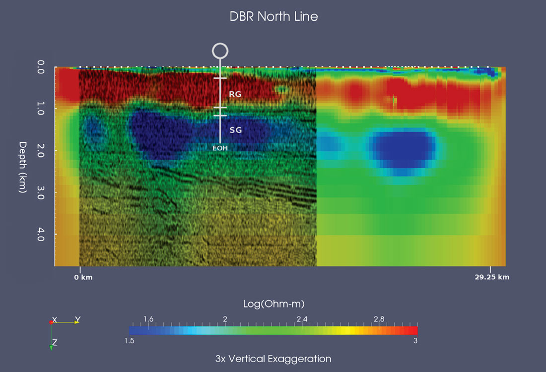
At 1167.5 m depth, Proterozoic mudstones of the Shaler group were noted in DBR-001, this correlates quite well with the moderately conductive layer (in blue) seen from approximately 1100 m to 2 km depth in the 3D TAMT inversion (Figure 8).

The near vertical offset seen in the seismic data at approximately 2.5 km depth, and the disrupted zone of reflectivity below, correlates quite well with a weakly conductive zone extending to depth in the 3D TAMT inversion (Figure 8). This is consistent with a zone of increased porosity due to fracturing, as is typical with faults. The tipper anomaly at this location also has a signature consistent with a weak linear conductor (a fault). A sudden termination of the Shaler mudstones occurs at the fault contact, which also corresponds to the edge of the magnetic anomaly (Figure 4) and the location of the maximum gradient in the gravity anomaly (Jefferson et al., 1994).

Further to the East, a layered series of East dipping reflectors correspond quite well with the top of a slightly more resistive zone (Figure 8), Vye (1972) interpreted these reflectors as the top of the intrusive body. From an EM perspective, we would expect to see an igneous intrusive as a resistive feature.

However, considerable ambiguity is present when one considers the regional presence of the Dismal Lakes group which typically underlies the Shaler Group. Comprising mostly carbonates, Dismal Lakes group would also be seen as a resistive feature from an EM perspective. But, the spatial association of fault structures with the character of the potential field data implies that the source of the East dipping reflectors (and the weakly resistive zone in Figure 8) are indeed contributing to the potential field anomalies (Jefferson, 1994).

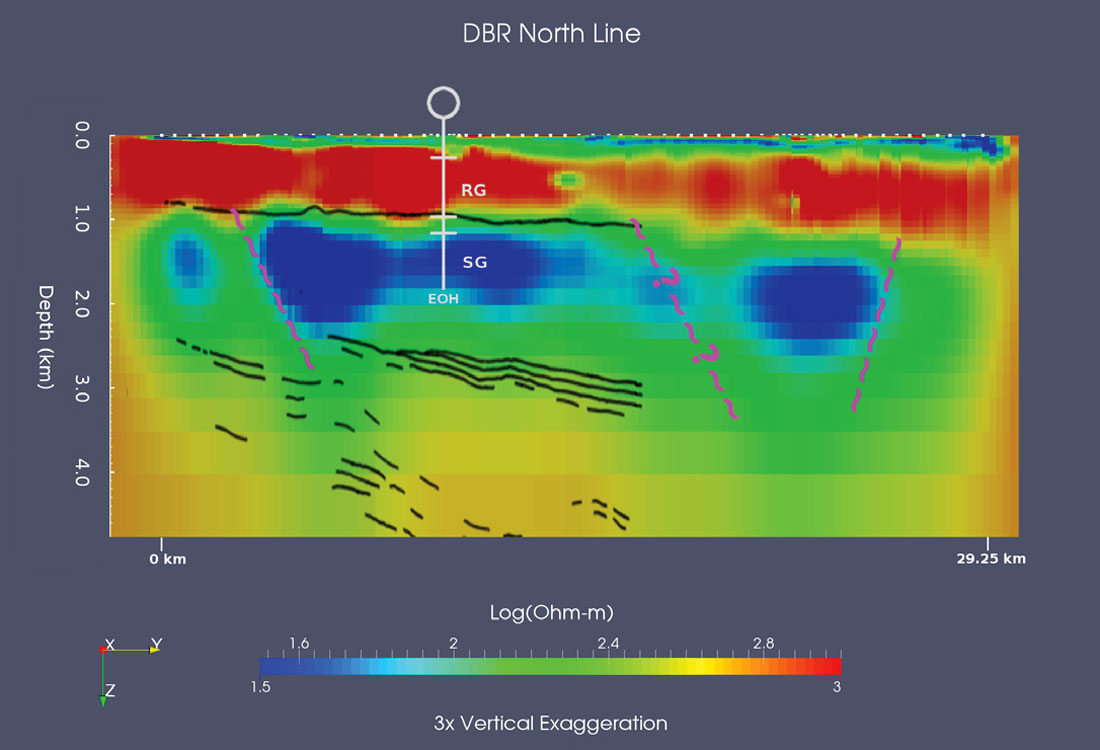
Past the eastern extent of the seismic data, it appears that the presumed intrusive body plunges with depth more rapidly and is offset once again by another fault. A 20 percent tipper anomaly, the largest on the property to date, is coincident with the abrupt lateral termination of Shaler mudstones near the East end of the TAMT survey line.

An interpretive overlay constructed by Hole and Isbell (1990) is shown on top of the 3D TAMT inversion in Figure 9, along with the location of inferred fault structures.

Conclusions

In agreement with Vye (1972), it appears that depth to the presumed intrusive body is on the order of 3.0 km. However, it is shallowest (2.5 km) at the West end of line, terminating or at the very least being offset vertically by fault structure. Further to the East, the presumed intrusive dips gradually to as deep as 3.2 km before it appears to plunge downward more rapidly. Near the East end of the TAMT survey line, indications of fault structure are present once again on the tipper, coincident with the abrupt lateral termination of Shaler mudstones.

Although Dismal Lakes group carbonates cannot be completely discounted as the source of the deep, weak resistive feature in the 3D TAMT inversion, and the East dipping layered reflectors from Vye (1972), it would appear to be less likely due to the spatial association of fault structures with the potential field anomalies.

However, until a drill hole is able to pass beyond approximately 3 km depth, it will still remain a question. Arguably, the best target would be the western-most extension of the presumed intrusive at its shallowest depth, targeting both the presumed body itself and associated fault structure.

We look forward to the completion of our third generation receiver with increased scope of application beyond uranium, base metal, gold, diamond and groundwater exploration.

¹ ELF – 3 Hz to 3 kHz, VLF – 3 kHz to 30 kHz

² Saturated near surface soils many times had a “jelly” like quality which was not very effective for coil burial.

³ Zxx, Zyy were generally very small, except in the infill areas at VLF (see Figures 6 and 7), and did not contribute significantly to the 3D inversion.

⁴ Note that drillhole DBR-001 was located approximately 1.5 km North of the survey line.

Acknowledgements

The authors would like to thank Darnley Bay Resources Ltd. for releasing the data for presentation, and in particular, Mr. Stephen Reford for explaining many of the historical aspects of the project. We would also like to thank Dr. Don Gendzwill for his many helpful comments and Mr. Bernie Maclean for making us aware of GSC Bulletin 575. Lastly, Dr. Martyn Unsworth for his editorial feedback and for initially making us aware of this special issue.