Multi-method geophysical prospecting of the Moviola lui Deciov archaeological site, Romania

Abstract

An archaeological geophysics survey was conducted on the Early Neolithic site of Moviola lui Deciov, in the Province of Banat, Romania. Magnetometry was used for the main prospection effort and a test of electrical resistivity imaging was conducted on a selected profile. In addition, magnetic susceptibility measurements were obtained from excavation pit samples.

The magnetic survey was successful in determining the extension of the site, in delimiting zones rich in structures and artefacts and in confirming the presence of a ditched enclosure that could prove to be the oldest known in the region. Detailed joint modelling of the magnetic and electrical response of the subsurface was used to confirm that electrical resistivity imaging can provide depth information to complement magnetic mapping.

One of very few archaeological geophysics projects reported in Romania, this survey paves the way for an increased use of geophysical techniques in the cultural heritage management of this country. From a methodological viewpoint, this work further demonstrates the potential of electrical resistivity imaging in archaeology.

Introduction

Moviola lui Deciov (Deciov’s knoll) is an Early Neolithic site in Western Romania (Banat Region). To date, very few archaeological geophysics surveys have been carried out and reported in Romania and the initial objectives of this study were mainly those typical of archaeological prospecting projects. Previous unpublished investigations and test excavations have revealed unambiguously the presence of a Neolithic, Star‹c̆evo-Köšršös-Criş occupation site but no clear appreciation could be deduced of how widespread the site was. The first objective was, therefore, to attempt to delineate the total extension of the site by mapping the abundance of anomalies that could be related to archaeological material.

An extremely enticing result of the test excavations was the discovery of evidences of a ditch feature possibly representing the trace of an enclosure surrounding the entire site. Although ditched enclosures are common features of Neolithic settlements (Whittle, 1994), they have never been found around sites of the period of Moviola lui Deciov. When present they are often very successfully mapped using geophysical techniques, particularly magnetometry (Tabbagh et al., 1988; Doneus and Neubauer, 1999). Another very important objective of this survey was, therefore, to attempt to confirm the presence of an enclosure completely surrounding the site and to map its characteristics.

From a methodological viewpoint it was also interesting to evaluate the potential benefits of using multiple techniques on such a site and to integrate their findings to achieve an understanding of the geophysical response beyond the m e re superposition of results of different origin. Magnetometry and area soil resistivity are used routinely for the mapping of archaeological sites. Although very efficient for fast and accurate mapping, these methods cannot in general provide an accurate image of the vertical distribution of archaeological materials. In many cases, archaeologists rely on georadar for precise depth determination. However, for sites such as Moviola lui Deciov, and, in fact, for the great majority of prehistoric sites located on agricultural land and devoid of stone structures, the presence of fine grained, clayey and moist soil and sedimentary material often precludes the use of georadar because of high signal attenuation. In these circumstances, direct current (DC) electrical resistivity imaging can provide the best and only alternative to georadar. This relatively recent technique is now widely employed in near-surface geological investigations. Although a few examples of archaeological applications have been reported (Noel and Xue, 1991; Sambueli et al., 1999; Neighbour et al., 2001), it still appears somewhat underutilized in this field. A test of this technique and how it could be utilized in a Central European Neolithic context constituted an important methodological objective of this work.

Archaeological Setting

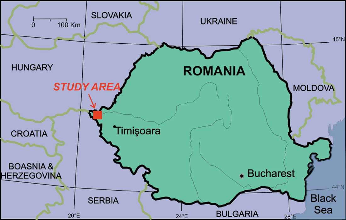
Moviola lui Deciov is a multicomponent Star‹c̆evo-Köšršös-Criş site in the southeastern periphery of the Great Hungarian Plain, within the Timiş province of Romania, just north of the Dudeştii Vechi village (Figure 1). This area has limited relief and generally lies below 100 m asl (Chapman, 1981). It was prone to periodic flooding prior to flood-protection works undertaken in the 20th century. Sedimentation from the periodic floods produced nutrient-rich soils, making the area attractive for early agriculture. The site is in a modern agricultural field and rises 3m over an area 200 m in diameter.

Moviola lui Deciov is an important stratified site first excavated by the local collector Nagy Gyula Kislegi in 1906 and 1907. These excavations resulted in the recovery of many complete artifacts currently located at Muzeul Banatului, in Timişoara, Romania. Recent test excavations in 2000 and 2001 identified two Starc̆‹evo occupations: 1) a lower occupation between 140 cm and 160 cm below the surface, consisting of a cultural floor of artifacts, charcoal, ash and fish scales; and 2) an upper occupation level between 95 cm and 110 cm below the surface, represented by a house floor feature and artifacts.

The discovery of the two Star‹c̆evo occupations makes Moviola lui Deciov an important site for a temporal analysis of culture change. Preliminary examination of pottery materials suggests an occupation period that encompasses the time frame of 5950- 5100 B.C. The site is also important because of the presence of a ditched enclosure. Future excavation will reveal the cultural association with this ditch, which at this time remains speculative. If this ditch is associated with the Starc̆‹evo-Criş occupation as the preliminary archaeological data indicate, it would be the earliest discovered in the region.

Data Acquisition and Results

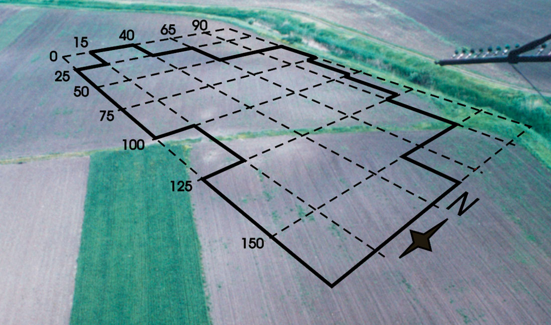
All measurements were collected with reference to the same grid (Figure 2), which consisted of individual survey lines oriented W-E and separated by 1 m. The spatial sampling interval along each line varied according to the method used. For most of the survey area, square sub-grids of 25 x 25 m were used and surveyed independently. In some cases rectangular sub-grids were used to achieve a more efficient coverage of the area. Three geophysical methods were employed for this study: magnetometry, electromagnetic conductivity (EM38) and DC electrical resistivity imaging. Electromagnetic surveying failed to reveal archaeologically significant anomalies and will not be discussed here. In addition to indirect surface measurements, we measured the magnetic susceptibility of a number of samples from test excavations. As a first step in the exploitation of the data, magnetic and electrical results are presented separately. The following section provides integration of the results.

Magnetic Survey

A total field proton precession magnetometer was used. In order to achieve maximum sensitivity, the sensor was held close to the ground, at a distance of 10-15 cm. The data were collected under a continuous acquisition mode by keeping a slow constant walking pace, corresponding to an average measurement interval of 0.20 m. A loop technique was used for diurnal corrections and a base station was re-occupied after walking two survey lines; a time interval of 4 min on average and never exceeding 6 min. To minimize the walking distances and the time intervals between successive base station readings, seven different base stations were used for the entire grid. These seven stations were tied together with 4.7 minutes separating the first and last reading. An area of 12,600 m² was covered by the magnetic survey.

The measurements were processed to obtain a complete map of the surveyed area. The first step was to apply a time-based correction to correct for temporal variations of the Earth’s magnetic field. This was done in the field for individual subgrids using their corresponding base station readings. An overall correction using the ties between individual base stations was applied later to reduce all measurements to a common datum. Due to the limited extent of the survey area and to the very flat topography, no other correction was needed.

Despiking removed most very large, short wavelength anomalies attributable to small, recent, iron-rich objects such as nails or fence wire lying at or very close to the surface. These objects were remarkably few in this particular agricultural field. Detrending and sub-grid boundary adjustments resulted in a seamless map of the surveyed area. Finally a light high-cut filter was applied to enhance the continuity of features.

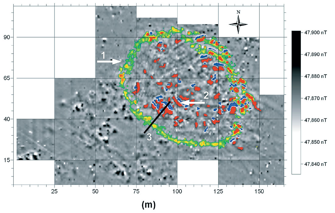
The final total field map is shown in Figure 3. Numerous anomalies are seen with a maximum range of variation of 65 nT. The distribution of anomalies defines very clearly the limits of the site, which does not appear to extend beyond the survey area . The most significant feature of the map is possibly the presence of an approximately oval positive anomaly, with a long axis measuring 80 m and a short axis measuring 62 m. This feature seems to surround completely the majority of smaller scale anomalies and it intersects the excavation trench where evidence of a ditch was found. It is, therefore, natural to interpret it as a ditched enclosure. This could constitute the most important archaeological contribution of this study, since such an enclosure would be the earliest discovered in this part of the world.

A number of high amplitude anomalies are also very interesting, e.g. at grid coordinates 90 m and 50 m (Figure 3). The test excavations have revealed the presence of burnt house features and magnetic susceptibility measurements of house material yield very large values consistent with large magnetic anomalies (see below). It is, therefore, likely that the largest anomalies, both in amplitude and extension, are created by house features, which will constitute targets of choice for future excavations.

All the other smaller scale anomalies almost certainly reveal the presence of archaeological features and artifacts such as individual ceramic objects, ovens, pits or house fragments. The pattern of anomalies in the southwest corner of the surveyed area, outside the oval enclosure, could be caused by more recent, possibly bronze age material.

Magnetic Susceptibility Measurements

The magnetic susceptibilities of soil and archaeological samples were measured in the laboratory using a Bartington MS2 meter and MS2B sensor. A total of 29 samples collected from the 2000 and 2001 test excavations were used. In addition, two hand samples of house material (daub), recovered during the 2002 geophysical survey, were subsequently sub-sampled for magnetic analysis.

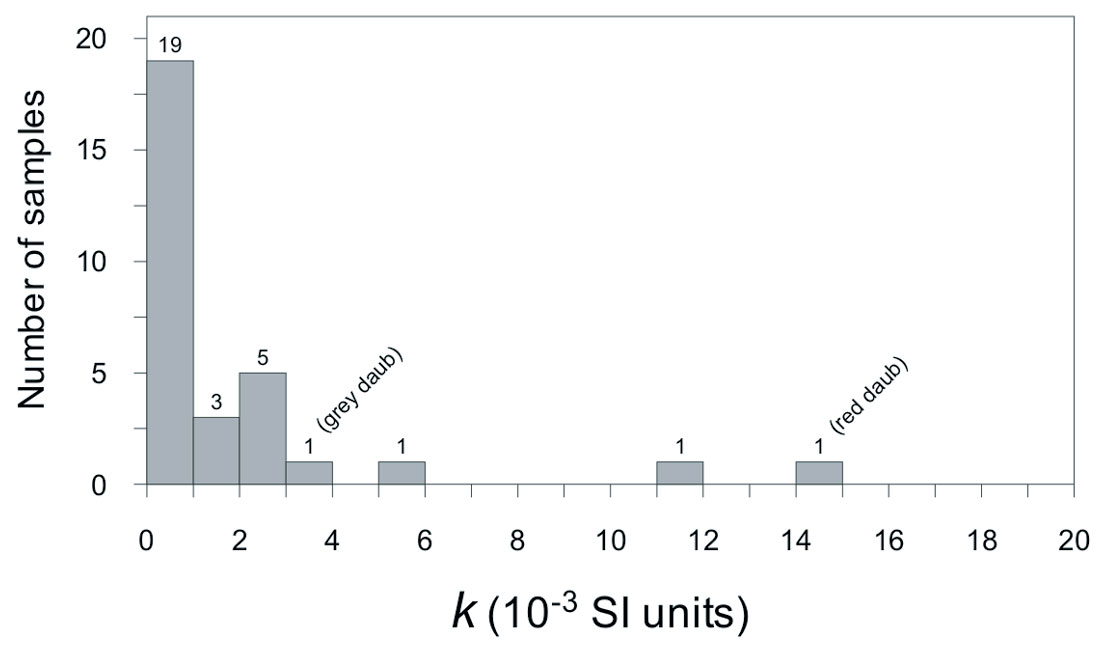
The results of these measurements are summarized in Figure 4 in the form of a histogram of values of low frequency volume specific magnetic susceptibility (k). The majority of soil samples have k values in the range 0.2 x 10^-3 to 1 x 10^-3 u.SI with some values reaching up to 3 x 10^-3 u.SI. One of the excavation samples containing reddish material suggestive of burning or archaeological debris has a large k of 11 x 10^-3 u.SI. The two daub samples have elevated but very different susceptibilities. The larger value corresponds to a mostly red sample with clear evidence of heating, while the weaker sample is mostly grey and probably essentially unmodified. The bulk of the soil samples provide an estimate of the background magnetic susceptibility between the surface and a depth of 2 m. The mean value for the 27 weakest samples (Figure 4) is 1.03 x 10^-3 u.SI. The daub samples and the more strongly magnetic excavation samples provide estimates of the k values for actual archaeological material. Although only four such samples are available, the results indicate that in this case k can vary between 3.7 x 10^-3 and 14.6 x 10^-3 u.SI. Because of the mode of sampling and the difficulty in extrapolating imperfect laboratory measurements to in-situ susceptibility values, these numbers represent only estimates. However, the differences between extreme values and the background value provide some useful constraints on the possible k contrast responsible for the magnetic anomalies detected and mapped by the surveys. These constraints will be used in a later section to reach a better understanding of the geophysical response of the materials present at the site.

Resistivity Imaging

A test of 2-D resistivity imaging was conducted to intersect prominent features along a profile selected on the basis of the preliminary results of the magnetic survey. A dipole-dipole array was used with a fixed 1 m potential and current dipole size and an inter-dipole separation varying from 0.5 m to 5 m. For each dipole separation, a measurement interval of 0.25 m was used to cover the entire profile. A total profile length of 24 m was acquired, yielding 383 data points and 10 data levels. Measured resistance values ranged from 0.659 to 11.559 Ω, well above the sensitivity of the instrument.

The dipole-dipole resistance measurements were converted to apparent resistivity and inverted into a resistivity model. The inversion was performed using RES2DINV (Loke and Barker, 1996). A good fit between observed and predicted apparent resistivities is easily achieved, which indicates a coherent data set with little noise. The reconstructed resistivity model and a tentative interpretation are shown in Figure 5. A generally high resistivity layer from approximately 0.3 to 1.5 m depth is readily apparent, with significant lateral changes in resistivity present within this layer. Below 1.5 m, lower resistivities typical of fine-grained sediment are found. Between 5 and 9 m along the profile, this lower resistivity layer is interrupted by a funnel-shaped higher resistivity zone extending at least down to the depth limit of the section (3 m).

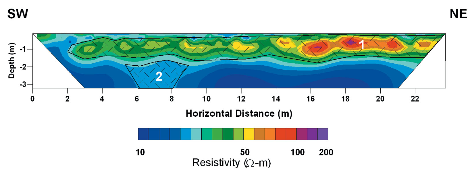
The profile was selected to intersect major magnetic anomalies and a brief comparison of resistivity image and magnetic map reveals that a very good correlation exists between high resistivity zones and magnetic anomalies. For comparison purpose, it is important to take into account that the positive peaks of magnetic anomalies are shifted towards the south relative to the actual location of the anomaly source in the ground. The highest resistivity values (15.5 to 21.5 m, horizontally) coincide with large magnetic anomalies previously attributed to house features. Therefore, the high resistivity top layer most likely corresponds to the layer of archaeological material which thus appears to extend down to about 1.5 m, in agreement with the test excavations. Perhaps most interesting of all, the horizontal position of the funnel-shaped resistivity zone exactly coincides with the position of the oval feature interpreted as an enclosure. A ditch dug into fine-grained clayey material and filled with coarse debris of various sizes would indeed be expected to have a higher resistivity than its surroundings. If this interpretation is valid, the resistivity section provides an estimate of the size of this feature. Based on the contoured resistivity model, it appears to have a maximum width of 3 – 4 m, and a depth below the surface of more than 3 m. These dimensions are quite comparable with other known Neolithic ditches.

Discussion and integration of results

A brief examination of the resistivity image and the corresponding magnetic profile has indicated that a very close correlation exists between the locations of high resistivity anomalies and the locations of magnetic anomalies. On archaeological sites it is generally safe to assign an anthropic origin to magnetic anomalies but resistivity variations may have a geologic origin in many cases. A way to evaluate the similarity of the anomaly sources is to compare the resistivity model resulting from inversion of electrical data with a magnetic property model obtained from magnetic field data.

Any geophysical model has two fundamental components: (1) a physical property component and (2) the spatial distribution of this property. To push further the integration, a magnetic model was built using susceptibility measurements for the physical property component and the geometrical characteristics of the resistivity model for the spatial distribution of susceptibility. In order to construct an initial model, the basic assumption was that high resistivities in the electrical image correspond to high susceptibility material in the magnetic model. In smooth models, such as those typically produced by electrical resistivity imaging, it is always hazardous to try to assign specific boundaries to subsurface features by identifying them with specific contour lines. In this case, the preliminary model was constructed by arbitrarily choosing the 43 Ω-m contour line for moderately elevated susceptibilities and the 73 Ω-m contour line for high susceptibilities. The presumed ditch was assumed to be represented by the 22.5 Ω-m contour line. The apparently needlessly precise numbers are due to the logarithmic scale used for contouring the resistivity image. The susceptibility values (k) were selected to be compatible with actual sample measurements. The initial model consisted of six bodies with k = 1 x 10^-3 u.SI and two bodies with k = 5 x 10^-3 u.SI.

In very shallow and high resolution surveys of this nature it is very important to consider carefully the reference of elevation used for data acquisition and for computing the models. It is especially important when attempting comparison and integration of results from different survey methods. In the case of the magnetic survey, the sensor was held at an average of 0.15 m above the surface of the ground. Allowing for the finite size of the sensor bottle, it is estimated that the measurements correspond to an elevation of 0.20 m above the surface of the ground. Therefore, the depths of the magnetized bodies in the model have to be decreased by the same amount to obtain their true distance from the surface.

In the case of the resistivity image the situation is less straightforward. In the image reconstruction process, it is assumed that the electrical sources (electrodes) are located at the surface of the ground, at a depth of 0 m. This is never quite true as electrodes have to be driven a certain distance into the ground. In addition, although most of the current flows from the tip of the electrodes, a very poorly known amount also emanates from their length. These effects make it very difficult to assign a precise depth reference to an electrical image. A difference of 0.1 to 0.2 m is negligible when a section of several tens of meters is reconstructed but when structures are imaged at a depth of about 1 meter it becomes very significant. Due to the very good ground contact at the site, the length of electrode buried into the ground could be kept at constant 0.15 m value. It is, therefore, estimated somewhat arbitrarily that a correction of 0.10 m has to be introduced in determining the depths of the magnetic bodies as inferred from the electrical image.

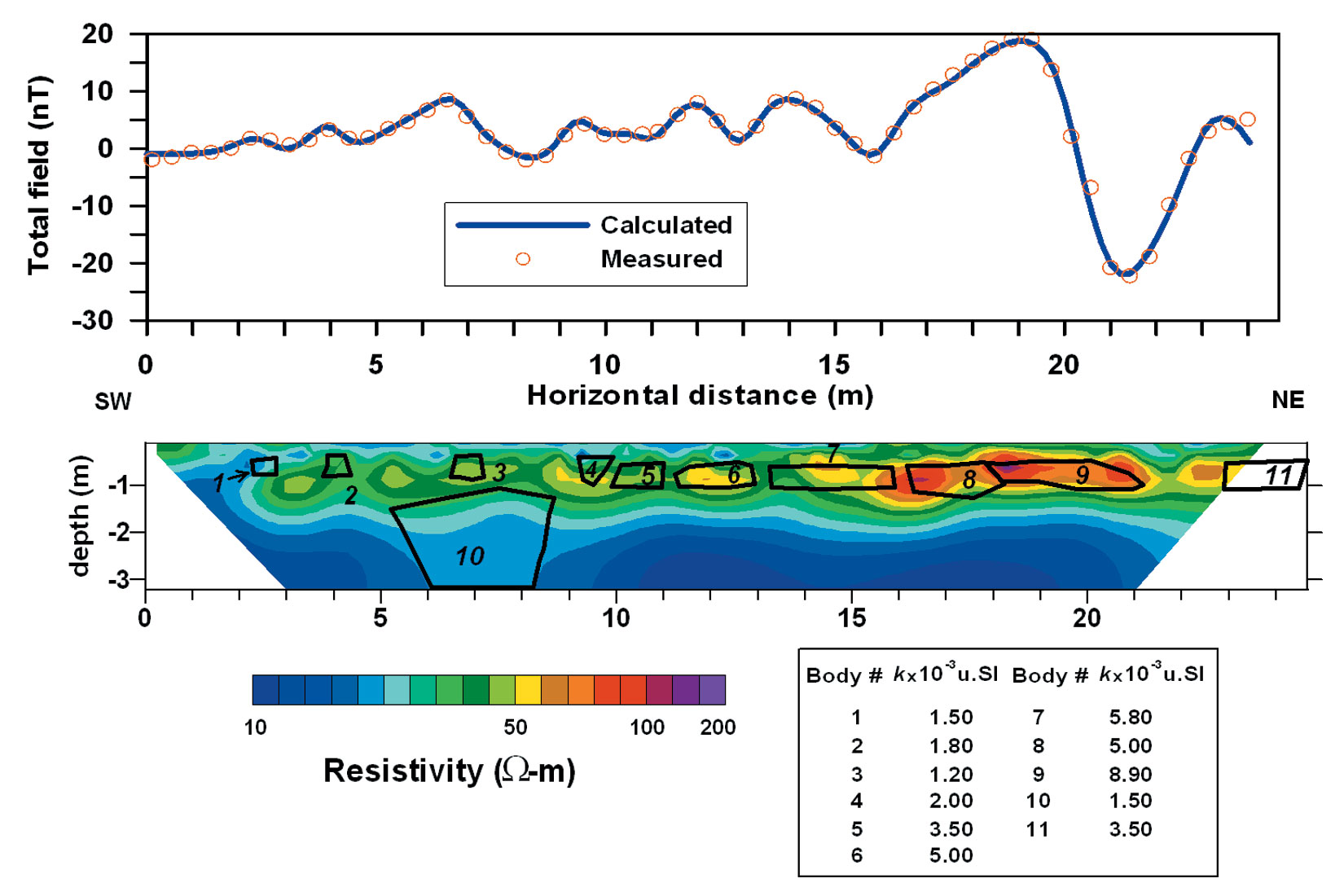
The magnetic response of the model was computed using a 2D magnetic modelling program that calculates the response of uniformly magnetized polygonal bodies. It was then matched with the observed magnetic profile extracted from the map. The first pass actually resulted in a good match for the horizontal position of the magnetized bodies and the overall trend of the magnetic anomalies. The major discrepancies concerned the amplitude and width of the individual anomalies. The fit between predicted and observed anomalous magnetic field values was then improved by adjusting both body shapes and susceptibility values in a standard approach. Two additional bodies on both ends of the section had to be added to achieve an excellent match. Figure 6 shows the final result in the form of superimposed resistivity image and magnetic model at the bottom and superimposed predicted and observed magnetic anomaly profiles at the top.

Caution must be used in comparing two subsurface models obtained with two very different techniques. The resistivity model is inherently smooth and gradual changes of resistivity can be assigned within the constraints imposed by the finite sizes of the mesh elements. On the contrary, the magnetic model is constrained to discrete polygonal bodies of constant magnetic susceptibility. In an archaeological context where one expects to find well delimited structures with strong physical property contrast relative to their sedimentary background, a polygonal model might in many cases be a closer representation of reality. The positive aspect of this disparity is that if similarities are found between the two models, despite their fundamentally different origins, they are almost certainly due to the underlying true geophysical characteristics of the subsurface.

Comparison of the two models reveals that, generally, good agreement between the locations of magnetized bodies and high resistivity zones is observed, which confirms that their sources are, for the most part, identical. A clear positive correlation between the resistivity and susceptibility is also observed, with the highest resistivities coinciding with the highest susceptibilities. These two results clearly demonstrate the complementary characteristics of the magnetic and electrical methods on the study site. It appears that resistivity imaging can be used effectively to determine the depth distribution of the structures mapped by magnetometry.

Some discrepancies between the two models also exist and a lot can be learned from them in order to better interpret resistivity images in general. The bodies in the magnetic model had to be made systematically thinner and more angular than in the initial model that attempted to follow resistivity contour lines. The features of the resistivity model are therefore broader and rounder than the modelled magnetic sources; this is exactly what would be expected since the resistivity inversion tends to produce a smooth model. This clearly illustrates why caution has to be exerted when assigning specific resistivity contours to subsurface features. In some locations, in particular from 13 to 16 m, the shape of the final magnetic body is completely different from the resistivity contour lines. In this case the likely explanation is that, although the locations of magnetic and electrical anomaly sources coincide, the spatial distribution of the two properties cannot be identical. Another interesting discrepancy is seen at the northeast end of the section, around 23 m, where the magnetic body is displaced from the resistivity anomaly by about 1 m laterally. This is most likely due to an edge effect in the resistivity inversion process. The two small bodies at the southwest end appear to correspond to a single relatively high resistivity zone occupying a deeper location. This could also be due to an edge effect or a lack of resolution of the resistivity method.

Two fundamental aspects of magnetic and resistivity modelling have not yet been considered. One is the role played by remanent magnetization in the magnetic model. The model predicts the response of a magnetized object but this magnetization can be either induced or remanent. Although it was not measured, it is quite clear that some of the material present at the site must posses a very significant remanent magnetization. Considering the age of the site (less than 7000 years BP) the directions of induced and remanent magnetizations are not very different for in-place features. For the fairly large, most likely in-place features considered in this modelling exercise, the consequence of neglecting the effect of remanent magnetization is, therefore, only to overestimate the susceptibility, which does not invalidate the predictions of the model.

The second important aspect of modelling that has to be considered is the consequence of modelling three-dimensional structures with a two-dimensional approximation. The strong anomaly sources present in the NE half of the profiles, when observed on the magnetic map, do not extend more than approximately 4 m on either side of the profile. A 2D approximation is therefore not really adequate, although the shallowness of the sources (less than 1 m) should limit the magnitude of errors. Due to their different physical basis, magnetic and electrical models are affected differently, with the stronger effect expected for the electrical model. Consequently, some discrepancies between the two models – and of course with the as yet unknown reality – are to be expected. However, this should not affect the main conclusions issued of the comparison between models.

Conclusion

From an archaeological prospective all the objectives have been met. The most useful results are provided by the magnetic map, with valuable depth information provided by the electrical resistivity imaging profile. The extension of the site has been well defined, which will greatly help for future investigation and conservation efforts. Numerous anomalies have been found; some are very strong with lateral extensions of several meters and represent priority targets for detailed excavations. Possibly the major contribution of the survey is the discovery of an oval anomaly surrounding the site, which helps build a very strong case for claiming the existence of a ditched enclosure at this early stage of the Central European Neolithic.

From a methodological perspective, some valuable information is obtained from the comparative analysis of the magnetic and electrical imaging surveys. The test of electrical resistivity imaging is quite successful and it demonstrates that this technique can be used advantageously to obtain depth information on archaeological sites with no stone structures. The joint modelling of electrical and magnetic data gives a unique insight into the origin of both kinds of anomaly and in this case it shows that their sources are mostly identical. This is an important result since it shows how complementary the two techniques can be, with magnetometry providing a fast mapping tool and electrical imaging supplying targeted depth information at key locations.

As always in archaeological geophysics studies, the ultimate feedback will be provided by subsequent excavations. The results presented here are being used to plan new targeted archaeological excavations of the site, and a completely exposed section corresponding to the test resistivity image will soon be available.

Numerous similar sites exist in western Romania and, as in all parts of the world, they are coming under increasing pressure from human development. This study will thus, we hope, contribute to imparting a new momentum for the use of geophysical techniques for the study, management and conservation of these sites.

Acknowledgements

The author gratefully acknowledges Joe Moravetz (Dept. of Archaeology, University of Calgary) and Dan Ciobotaru (Direction of Culture, Cult and National Cultural Heritage of Timis, Romania) for initiating the project, providing access to the site and contributing to data acquisition and archaeological interpretation. They will also carry the burden of verifying the geophysical results. Dominique Cossu contributed to data acquisition and drafted some of the figures. This project was made possible through the logistical support of Museum of Banat, Timişoara, and through an International Project Grant from the University of Calgary. All the field project participants are deeply thankful to the Kalcov family and the citizens of Dudestii Vechi for a wonderful welcome.