Joint simultaneous inversion of PP and PS angle gathers

Abstract

We present a new approach to the joint simultaneous inversion of PP and PS angle gathers for the estimation of Pimpedance, S-impedance and density. Our algorithm is based on three assumptions. The first is that the linearized approximation for reflectivity holds. The second is that PP and PS reflectivity as a function of angle can be given by a set of linearized equations. The third is that the background trend can be described by a linear relationship between the logarithm of P-impedance and both S-impedance and density. Given these three assumptions, we show how a final estimate of P-impedance, S-impedance and density can be found by perturbing an initial low-frequency model. After a description of the algorithm, we then apply our method to both a synthetic and real data set.

Introduction

The goal of pre-stack seismic inversion is to obtain reliable estimates of P-wave velocity (V_P), S-wave velocity (V_S), and density (ρ) from which to predict the fluid and lithology properties of the subsurface of the earth. One solution to this problem was discussed by Russell et al. (2006) in a special edition of the Recorder, which was based on the SEG expanded abstract by Hampson et al. (2005). Figure 1, taken from Russell et al. (2006) shows the fundamental seismic concept behind pre-stack inversion, in which we show the mode-converted reflected and transmitted waves from an incident seismic P-wave at the boundary between two elastic layers in the subsurface of the earth, with an incident angle equal to θ₁.

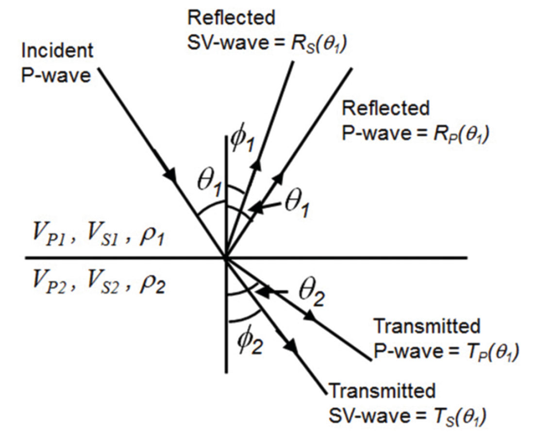
The computation of the amplitudes of the reflected P and Swaves was first solved by Zoeppritz (1919). Using the Zoeppritz equations, and a knowledge of the angle of incidence of the input P-wave as well as the velocities and densities of the two layers (noting that the other angles can be computed using the angle of incidence and the velocities using Snell’s law), we can easily perform forward modeling at the layer boundary to compute the amplitudes of the reflected and transmitted waves. This can also be generalized to multiple layers for both the primaries-only case and also the more complete case in which transmitted, converted and multiple reflections are taken into account (Fuchs and Müller, 1971, Kennett, 1983). However, the inverse problem of finding the velocities given the amplitudes is much more difficult than the forward problem, given the nonlinear nature of the Zoeppritz equations. For that reason, Hampson et al. (2005) perform pre-stack inversion by starting with the linearized Aki-Richards equation (Aki and Richards, 2002, Richards and Frasier, 1976) which was re-formulated algebraically by Fatti et al. (1994) as

where c₁=1+tan²θ , c₂= –8γ²sin²θ , γ=V_S/V_P , c₃= –0.5tan² θ+²γ²sin²θ , and the linearized P-reflectivity (R_P), S-reflectivity (R_S) and density reflectivity (R_D) are given by

It should be pointed out that the inversion problem was also discussed by Simmons and Backus (1996), who inverted for the linearized P-reflectivity (R_P), S-reflectivity (R_S) and density reflectivity (R_D) terms of equations 2 through 4, using the Aki- Richards linearized approximation of equation 1. Simmons and Backus (1996) also assumed that ρ and V_P are related by Gardner’s relationship (Gardner et al. 1974), given by

and that V_S and V_P are related by Castagna’s equation (Castagna et al., 1985), given by

The authors then use a linearized inversion approach to solve for the reflectivity terms given in equations 2 through 4.

Buland and Omre (2003) use a similar approach which they call Bayesian linearized AVO inversion. Unlike Simmons and Backus (1996), their method is parameterized by the three terms, ΔV_P /V_P, ΔV_S /V_S, and Δρ/ρ, again using the Aki-Richards approximation. The authors also use the small reflectivity approximation to relate these parameter changes to the original parameter itself, or

where ln represents the natural logarithm. Similar terms can be given for changes in both S-wave velocity and density. This logarithmic approximation allows Buland and Omre (2003) to invert for velocity and density, rather than reflectivity, as in the case of Simmons and Backus (1996). Hampson et al. (2005) inverted directly for the P and S-impedance terms and density, using a similar small reflectivity approximation to the one used by Buland and Omre (2003). They also used modified relationships similar to those of equations 5 and 6.

In the present study, we extend the simultaneous inversion method presented by Hampson et al. (2005) to the joint inversion of PP and PS gathers, so we refer to the method as joint simultaneous inversion. In the next section we will start by reviewing post stack inversion, then we will review the full theory of prestack PP simultaneous inversion, and then we will extend the method to PP and PS data.

Theory

We start by reviewing the principles of model-based post-stack inversion (Russell and Hampson, 1991). First, by combining equations 1 and 7, we can show that the small reflectivity approximation for the P-wave reflectivity is given by

where i represents the interface between layers i and i+1. If we consider an N sample reflectivity, equation 8 can be written in matrix form as

where L_Pi = ln(Z_Pi).

Next, if we represent the seismic trace as the convolution of the seismic wavelet with the earth’s reflectivity, we can write the result in matrix form as

where S_i represents the i^th sample of the seismic trace and w_j represents the j^th term of an extracted seismic wavelet. Combining equations 9 and 10 gives us the forward model which relates the seismic trace to the logarithm of P-impedance:

where W is the wavelet matrix given in equation 10 and D is the derivative matrix given in equation 9. If equation 11 is inverted using a standard matrix inversion technique to give an estimate of L_P from a knowledge of S and W, there are two problems. First, the matrix inversion is both costly and potentially unstable. More importantly, a matrix inversion will not recover the low frequency component of the impedance. An alternate strategy, and the one adopted in our implementation of equation 11, is to build an initial guess impedance model and then iterate towards a solution using the conjugate gradient method.

We can now extend the theory to the pre-stack inversion case. For a given angle trace S(θ) we can therefore extend the zero offset (or angle) trace given in equation 11 by combining it with equation 1 to get

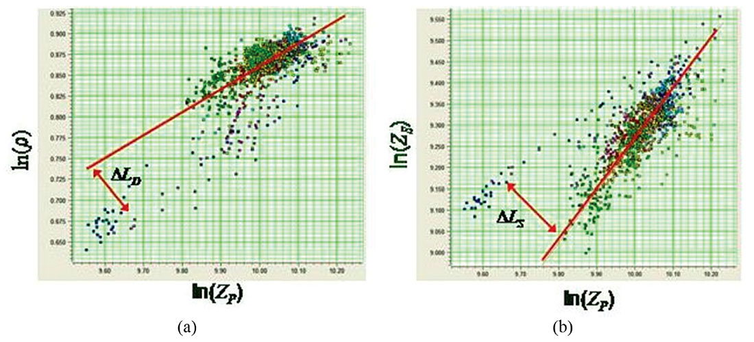
where L_Pi = ln(Z_S) and L_D = ln(ρ). Note that the wavelet is now dependent on angle. Equation 12 could be used for inversion, except that it ignores the fact that there is a background relationship between L_P and L_S and between L_P and L_D. Because we are dealing with impedance rather than velocity, and have taken logarithms, our relationships are different than those given by Simmons and Backus (1996) and are given by

and

That is, we are looking for deviations away from a linear fit in logarithmic space. This is illustrated in Figure 2.

Combining equations 12 through 14, we get

where

(Note that when we differentiate equations 13 and 14, the constant terms k_c and m_c go to zero and are therefore not present in equation 15). Equation 15 can be expressed in matrix form as

If equation 16 is solved by matrix inversion methods, we again run into the problem that the low frequency content cannot be resolved. A practical approach is to initialize the solution to [L_P ΔL_S ΔL_D]^T = [ln(Z_P0) 0 0]^T, where Z_P0 is the initial impedance model, and then to iterate towards a solution using the conjugate gradient method.

We will now extend the previous derivation to include pre-stack converted-wave measurements (PS gathers) that have been converted to PP time. We will use the linearized form of the equation that was developed by Aki, Richards, and Frasier (Aki and Richards, 2002, Richards and Frasier, 1976). It has been shown by Margrave et al. (2001) that this equation can be written as

where

and

The reflectivity terms R_S and R_D given in equation 17 are identical to the terms given in equations 3 and 4. Using the small reflectivity approximation, we can therefore re-write equation 17 as:

Next, using the relationships between S-impedance, density and P-impedance given in equations 13 and 14, equation 18 can be further re-written as

where

Note that equation 19 allows us to express a single PS angle stack as a function of the same three parameters given in equation 15. Also, equation 19 is given at a single incident angle θ. When we generalize this equation to M angle stacks, we can combine this relationship with equation 16 and write the general matrix equation as

Equation 20 gives us a general expression for the simultaneous inversion of N PP angle stacks and M PS angle stacks. Note that we extract a different wavelet for each of the PS angle stacks, as was done for each of the PP angle stacks.

Model Example

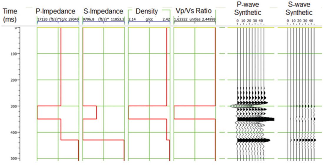
We will now apply this method to a model data example, shown in Figure 3. The model for these inversion tests is the Ostrander model (Ostrander, 1984), which consists of a gas sand between two identical shales, in which both the V_P /V_S ratio and acoustic impedance of the gas sand are less than that of the shales (this is called a class 3 AVO anomaly). The synthetic data is calculated using the Aki-Richards equations given in equations 1 (for the PP synthetic) and 17 (for the PS synthetic). Traces are modeled from 0 to 45 degrees. For the display shown in Figure 3, the PS data has been converted to PP time. The wavelet is a band-pass filter with cutoff frequencies of 5/10-50/60.

The reason for using such a simple synthetic example is that we know exactly what the correct answer is, so that as we vary the key parameters in the inversion we can quantify the effect of these parameters on the inversion result. In particular, we have found two issues which can affect the inversion result:

1. Constant gamma (V_S / V_P ratio) versus variable gamma, and
2. Whether the PS data has been transformed to PP time or left in the original PS time.

We will address both of these issues in the following tests. For point number 1, note that the scaling terms c₂ and c₃ in equation 1 and c₄ and c₅ in equation 17 are dependent on γ, the V_S / V_P ratio, and that this ratio should vary as a function of depth or time. Thus, approximating this ratio as a constant for the sake of stability in the algorithm will actually produce a slightly incorrect result. In our first implementation of this method, the variable γ was assumed to be constant and supplied by the user. A second approximation in this implementation was that the angle θ was taken as the incident angle, when actually it should be the average between the incident and transmitted angle, as discussed above. As just mentioned, the motivation for both of these approximations was that they allowed the c terms to be constants with time, which sped up and stabilized the calculation. To address these problems, we therefore added an option to calculate γ automatically instead of letting the user input the value. When this option is used, the following things happen:

1. A time-variant gamma is calculated from the initial guess model and used to start the inversion.
2. Every five iterations during the inversion process, the timevariant gamma is updated with the current values from the inversion. This is an approximate solution to the non-linear problem created with one of the “unknowns” being in the coefficients.
3. The correct average angle is used for all calculations, using the current time-variant velocity.
4. The process runs much slower than the constant gamma assumption.

To illustrate the difference between constant and variable values of gamma, Figure 4 shows the results on the logs of inverting the synthetic using a constant value of γ = 0.5. The figure shows the results (in red) after 50 iterations, starting from a smooth initial guess (shown as the smooth black line). The correct answer is shown as the blocky blue line on the same plot as both the initial guess and the final result. Before the inversion, the PS data had been transformed to PP time.

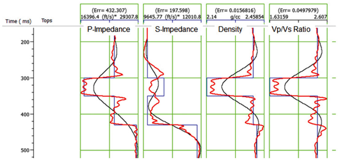
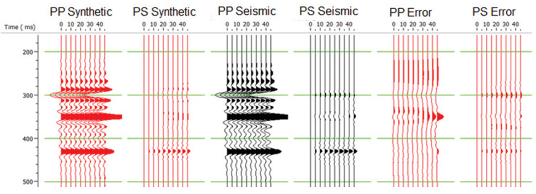
In Figure 4, it is obvious that the final result is reasonably good but not exact, and is different on each well log. The fits to the P-impedance, density and V_P / V_S ratio are actually much better than the fit to the S-impedance, where there is an obvious decrease, rather than increase, in the gas sand (that is the event between 300 and 350 ms). To quantify the fit, the RMS error has been written at the top of each well log. Note that the P-impedance has an RMS error of 432 (m/s)*(g/cc), the S-impedance has an RMS error of 197 (m/s)*(g/cc), the density has an RMS error of 0.015 (g/cc) and the V_P / V_S ratio has an RMS error of 0.049. Figure 5 shows the synthetic seismogram results from inverting the synthetic using a constant value of γ = 0.5. The figure shows the PP and PS synthetics on the left in red, the PP and PS original seismic gathers in the centre in black, and the PP and PS error in red on the right, where the error was computed by subtracting the seismic gathers from the synthetic gathers. Notice that the PP error is largest on the event at 350 ms at the far offsets and that the PS error is largest at the deepest event and is fairly uniform across all offsets.

Next, Figure 6 shows the results on the logs of inverting the synthetic using a variable value of γ. The figure shows the results (in red) after 50 iterations, starting from a smooth initial guess (shown as the smooth black line). The correct answer is shown as the blocky blue line on the same plot as both the initial guess and the final result. Before the inversion, the PS data had been transformed to PP time. This time, the fit to all four logs is quite reasonable visually, and the fit to the S-impedance after inversion shows a much improved response through the gas sand zone. Again, we have quantified the fit by posting the RMS errors at the top of each well log. As expected, the error on the S-impedance has dropped dramatically. However, the error on the other three logs after inversion has gone up.

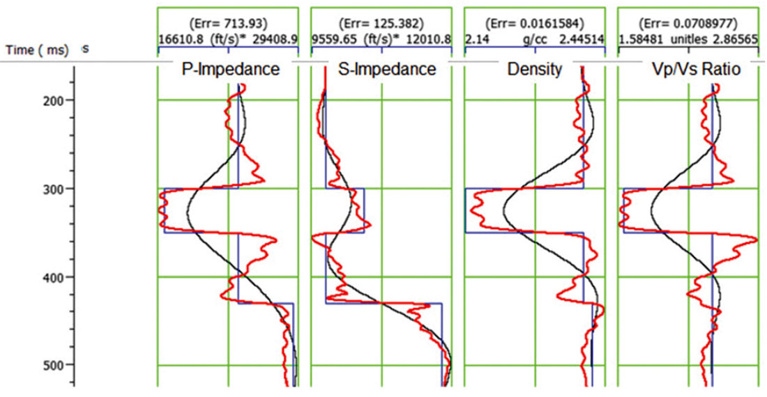
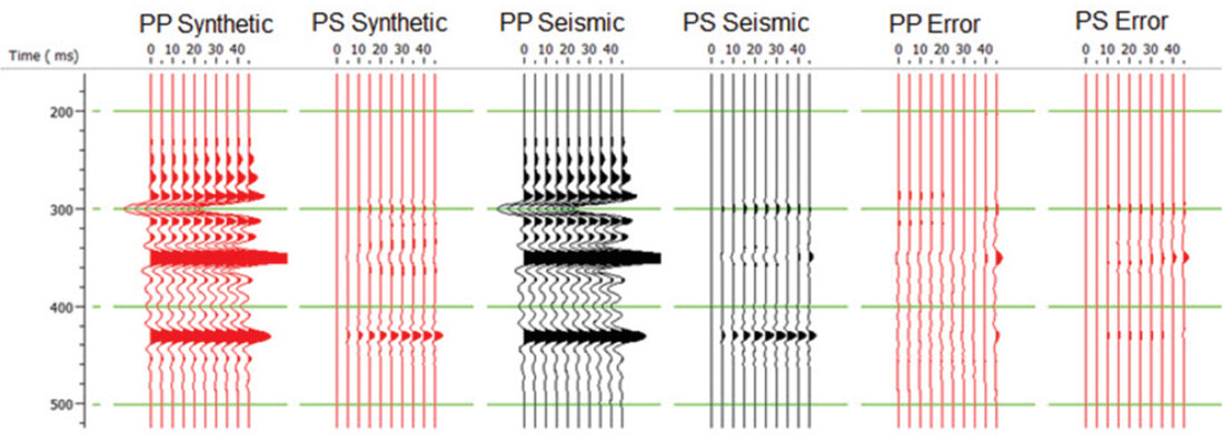
Figure 7 shows the synthetic seismogram results from inverting the synthetic using a variable value of γ. The figure shows the PP and PS synthetics on the left in red, the PP and PS original seismic gathers in the centre in black, and the PP and PS error in red on the right, where the error was computed by subtracting the seismic gathers from the synthetic gathers. Notice that when compared with Figure 5, the data error using a constant gamma value, the error has been dramatically reduced, especially at the far offset.

Next, we will turn our attention to the second problem identified above, which is whether the PS data has been transformed to PP time or left in the original PS time. Our inversion code so far has assumed that the PS data has been converted to PP time. This was convenient for a variety of reasons. However, the transformation of the PS data to PP time is generally a stretch/squeeze process, unless we have the unrealistic case of constant V_P / V_S ratio background. This produces an effective time-variant wavelet, as pointed out by Gaiser (2013). The current implementation approximates the time-variant wavelet by a constant wavelet extracted from PS data in PP time. An alternate formulation leaves the PS data in PS time, and performs the inversion on both data sets simultaneously. This is illustrated in Figure 8, in which the two synthetics are shown on the left side of the figure in PP time and are shown on the right side of the figure in PP and PS time, respectively.

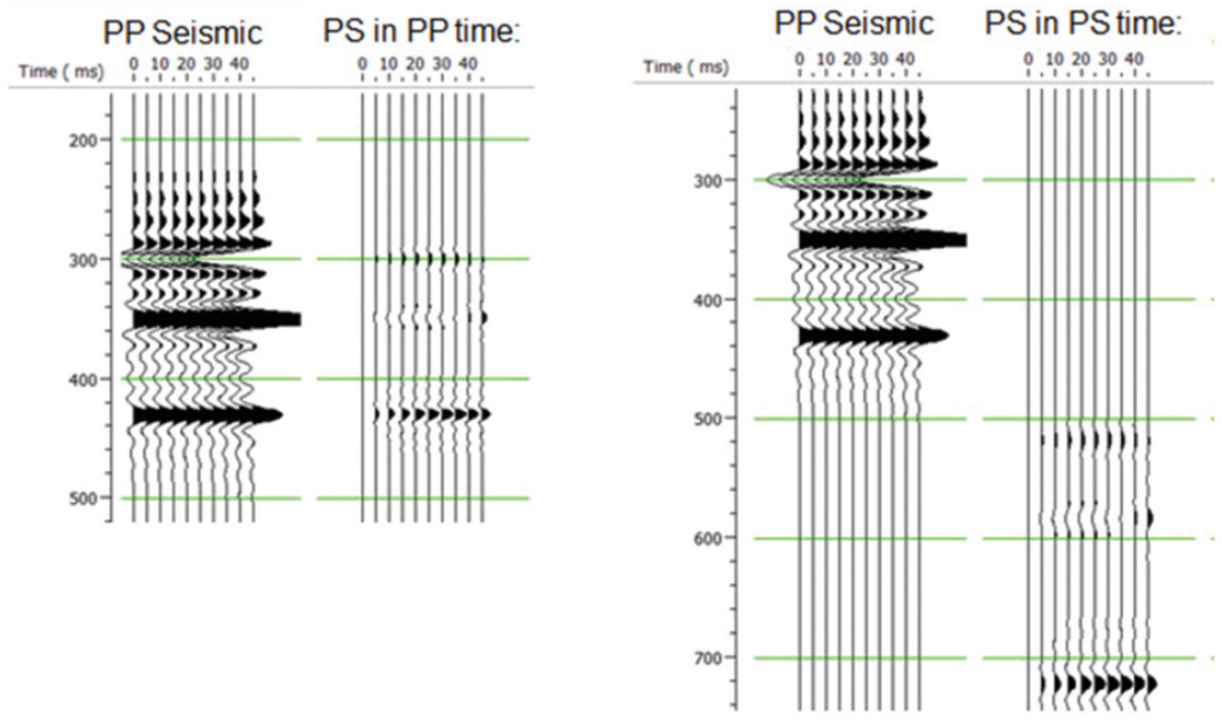
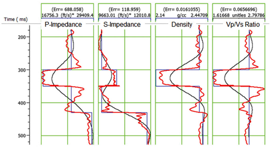
Figure 9 shows the results on the logs of inverting the synthetic using PP time for the PP data and PS time for the PS data. The figure shows the results (in red) after 50 iterations, starting from a smooth initial guess (shown as the smooth black line). The correct answer is shown as the blocky blue line on the same plot as both the initial guess and the final result. The fit to all four logs is quite reasonable visually, and the fit to the S-impedance after inversion shows the best response through the gas sand zone of all of our tests.

Again, we have quantified the fit by posting the RMS error at the top of each well log. This shows a drop in error on all four logs from the result in Figure 6. Our conclusion is that leaving the PS data in PS time gives an improved result, as predicted by the theory. However, the run-time can be significantly longer.

PP-PS Data Example

In this real data example, we will show a joint PP-PS inversion using a case study from northeastern Alberta. The workflow for this example involved the following steps:

1. Correlate the PP and PS data to wells
2. Pick the corresponding horizons on both datasets.
3. Use horizon based event matching to establish the mapping between PP and PS time.
4. Invert PP and PS data using simultaneous inversion.

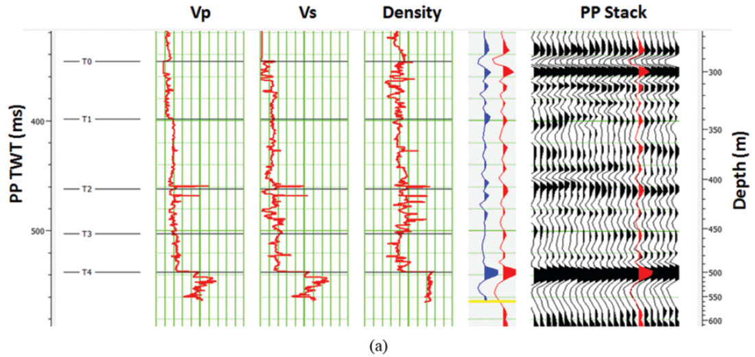
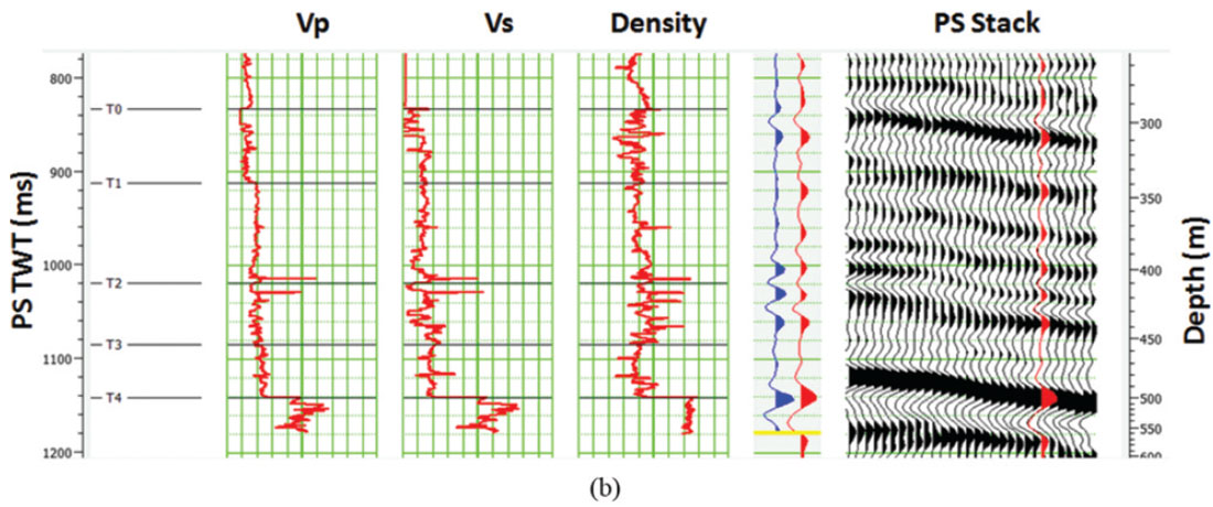
Figure 10(a) shows the correlated PP data and Figure 10(b) shows the correlated PS data from our example, where the V_P, V_S, and density logs are shown on the left of each figure, and the stacked data (PP or PS) is shown on the right. The synthetic trace (blue) to seismic trace (red) correlation is shown between the logs and the stacked data. Note that the ties are quite reasonable in both cases shown. The wavelets used to create the synthetic were extracted from the seismic data.

Finally, we applied joint inversion to this real dataset from Alberta, using the theory discussed in earlier in this paper. In this case we have only two inputs: the PP stack and the PS stack. We assume that the PP stack is equivalent to a PP angle gather at zero degrees and that the PS stack is equivalent to a PS angle stack at 15 degrees. The value of 15 degrees was arrived at by cross-correlating the traces in the PS stack with model traces at various angles and selecting the maximum correlation angle.

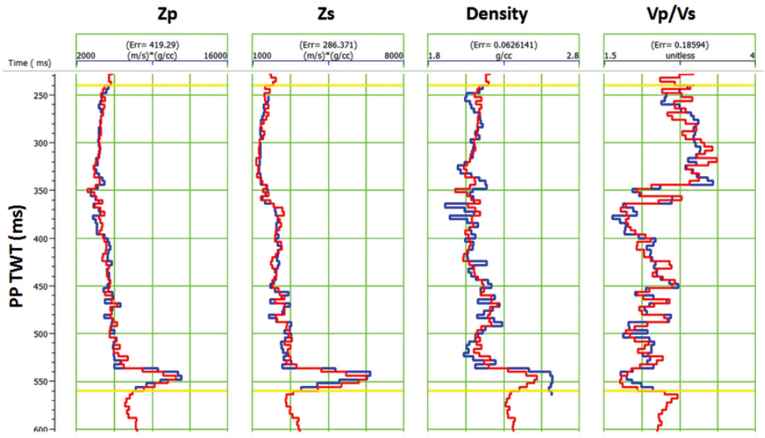
The quality of the inversion was evaluated by displaying inversion results at the well location overlaid on the corresponding real log curves. Figure 11 shows an example of such a display. Here, we are displaying P-impedance, S-impedance, Density, and V_P / V_S ratio. In each case, the real log is in blue, while the inversion result is in red. At the top of each track, the RMS error, the average difference between the real and estimated logs, is listed. For example, we can see that the average error in Pimpedance is 419 (m/s)*(g/cc).

In total, four different inversions were run to test the parameters described in the previous section:

1. Variable background gamma (Vs/Vp) with the PS data transformed to PP time.
2. Variable background gamma (Vs/Vp) with the PS data in its original PS time.
3. A constant background gamma (Vs/Vp = 0.6), with the PS data in PP time.
4. A constant background gamma (Vs/Vp = 0.6), with the PS data in PS time.

The constant background gamma of 0.6 was selected as the best from a series of test values for this parameter.

For each inversion test, the RMS errors were calculated at the well location using the method described in Figure 11. These results are tabulated in Figure 12, showing the errors for the estimated Zp, Zs and Density. For each case, the error is the RMS difference between the real curve and the inverted curve.

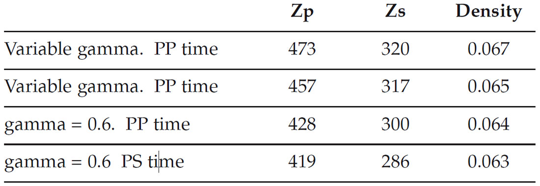
The test cases in Figure 12 are ordered with decreasing error, or improved inversion result, from top to bottom. We can see that performing the inversion with the PS data in PS time is consistently better than transforming the PS data to PP time. This conforms with the theoretical expectation. On the other hand, surprisingly, the variable gamma tests are not as good as the constant gamma of 0.6. This probably means that the actual V_P / V_S background is slowly varying and different from that calculated from the initial model.

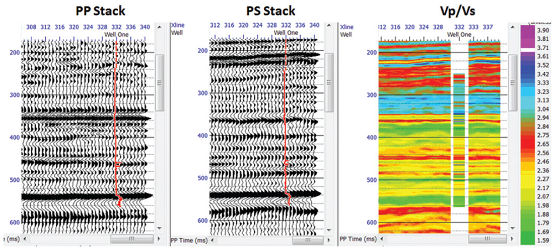
The result of applying joint inversion to the seismic datasets is shown in Figure 13, where we are displaying the inverted V_P / V_S ratio. Note that the V_P / V_S ratio in colour on the inserted well log matches the colour on the inversion results quite well. The colour scale in shown on the right hand side of the plot.

Conclusions

We have presented a new approach to the joint simultaneous inversion of pre-stack seismic data which produces estimates of P-impedance, S-Impedance and density. This method allows us to incorporate both PP and PS data into the solution, if we have first calibrated both datasets. The method is based on three assumptions: that the linearized approximation for reflectivity holds, that reflectivity as a function of angle can be given by the Aki-Richards equations, and that the background trend can be described by a linear relationship between the logarithm of Pimpedance and both S-impedance and density. Our approach was shown to work well for a modelled gas sand and for a joint PP-PS dataset from northeast Alberta. In the first example, prestack PP and PS synthetic data was used. In the joint PP-PS dataset the prestack data was not available and we applied the method to full stacks.