Interpreting seismic data in the presence of azimuthal anisotropy; or azimuthal anisotropy in the presence of the seismic interpretation

Measuring P-wave azimuthal anisotropy has been in the recent past an elusive task; therefore, the interpreter ignored this attribute of the seismic data and left the subject to the research and technology group geophysicists. Conversely, the interpreting geophysicist knew that when measured, the anisotropy could yield important reservoir properties related to fractures and stress fields. However, little did we suspect that P-wave azimuthal anisotropy both in velocity and AVO would change our perception of data interpretation as is happening now.

Two very important changes recently occurred in P-wave anisotropy research. First, very accurate methods of measuring both azimuthally varying velocity and AVO have been developed (Jenner, 2001 and Williams and Jenner, 2001 see for example the paper by Jenner in the August 2002 Leading Edge). Second, the very large anisotropy values published in the literature were found to be fairly normal and ubiquitous for basins that are not under primary burial. (See the suggested readings for P-wave velocity anisotropy magnitudes.) Therefore, understanding the anisotropy becomes a prerequisite to both obtaining the correct imaging from processing and determining the effects of the anisotropy on the conventional seismic interpretation. An interpreter will also find there is no escaping an anisotropic world even when not working with true 3-D data. The truth is, the earth does not care which tools we use, it still knows that it is anisotropic.

True 3-D data, wide azimuth, are data shot with a complete compliment sampling of source-receiver azimuths between the source and receiver with the additional requirement that offsets are fully populated in each azimuth class. These are the data that are appropriate for very accurate measurements of azimuthal velocity and azimuthal AVO. However, most data are not acquired in this way especially in the marine environment. Therefore, little can be done to directly view the anisotropy of the earth with these data. One might then say, no problem exists, concluding that there is no need to think about the anisotropy. However, opportunity exists in 2-D and narrow azimuth data to see the effects of azimuthal anisotropy and, when the interpreter realizes the effects, more insightful interpretations are available.

Azimuthally varying velocity

Azimuthally varying velocity is probably the most significant property of the seismic data that affects the seismic interpretation. A stacking velocity that varies with azimuth creates a list of issues for the interpreter:

• Loss of frequency content in stacking
• Character degradation of events
• Laterally varying non-geologic amplitude changes in the stacked data
• Poor fault resolution
• AVO signatures that degrade near faults
• Amplitude and phase footprints in 3-D data and with 4-D comparisons
• Poor merge seams between data sets
• Incorrect azimuthal AVO analysis
• Poor interval velocity resolution
• Velocity function misties at the intersections of 2-D lines.

And questions for the interpreter:

• Were the data migrated with the correct velocity field?
• Do the RMS velocities represent bulk rock velocities? (Can these velocities be used for acoustic inversion and depth conversion)??)
• Can workable land AVO measurements be correct? Can land AVO be sufficiently accurate to delineate reservoirs, fluids and fractures?

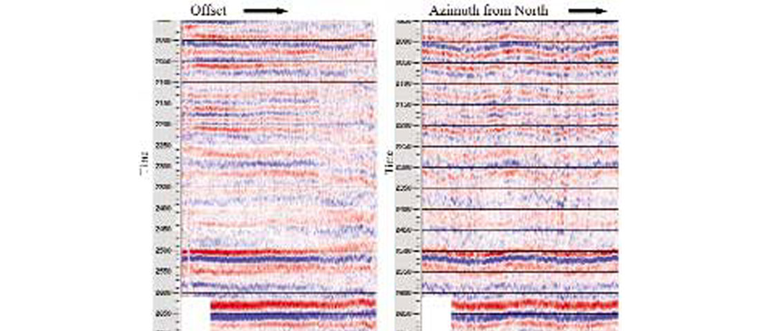
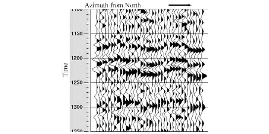
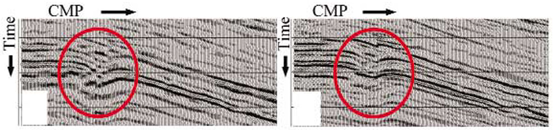
To take just one of the effects of azimuthally varying velocity, let’s look at the mis-stacking issue. Mis-stacking is the cause of the first seven points listed above. As an example, Figure 1 shows a common midpoint (CMP) sorted into offset. The far offsets are then sorted by azimuth. In the offset sort (Figure 1a), the CMP shows apparent reflector degradation with offset. When the far offsets are sorted by source-receiver azimuth from north, the apparent reflector degradation is seen as a set of time delays associated with changing velocity as a function of azimuth. It is the time shifts that create all the processing and interpretation issues, especially if the anisotropy changes quickly in a spatial sense. Figure 2 shows another azimuth sorted CMP where peaks and troughs are being stacked together.

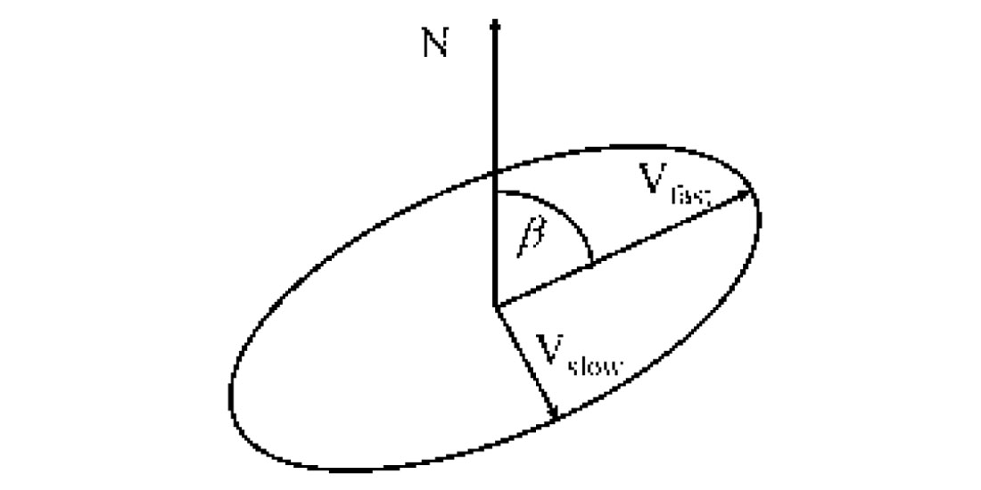
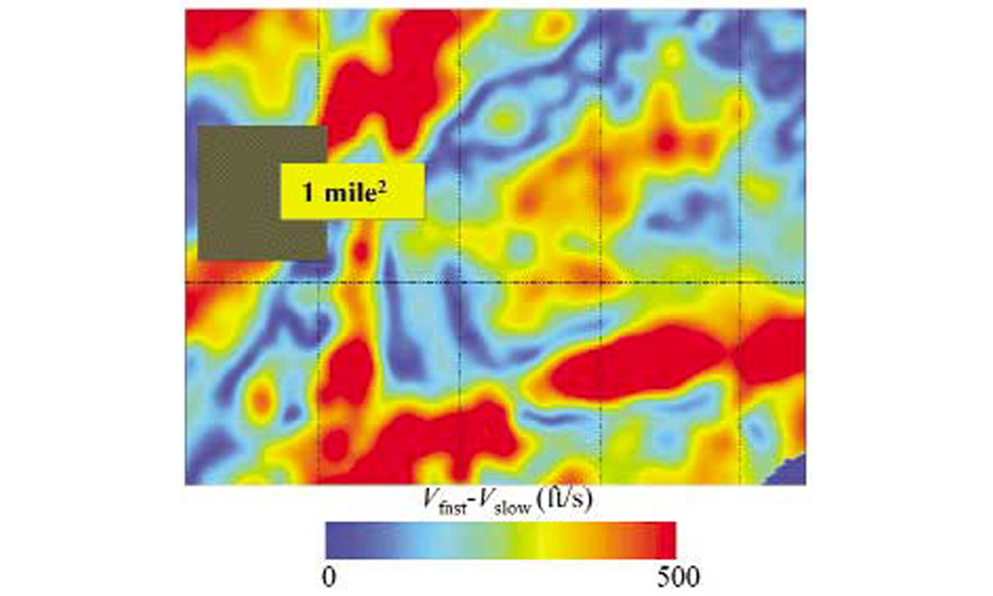
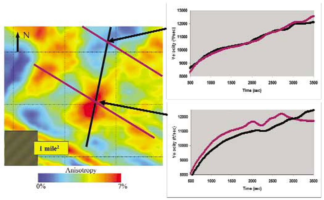
The azimuthal variation in NMO velocity observed in Figures 1 and 2 can be described by an ellipse in the horizontal plane (Figure 3). For a single set of vertical fractures, the fast velocity will be equal to the bulk rock velocity and will be orientated parallel to the fractures. When near a fault, however, multiple fracture directions are often observed. With these multiple directions of anisotropy, multiple ellipses are superimposed, often significantly reducing the seismically observed velocity. However, in this case the fast velocity will no longer represent the bulk rock velocity and may not be aligned to any of the fracture directions. In addition, Rapid change in fracture intensity, particularly near faults, can cause very rapid changes in the velocity field (Figure 4). Therefore, unless one is willing and able to pick very detailed velocity analyses, there are going to be areas in the data that mis-stack and these areas will more than likely be in proximity to the faults.

Now the interpreter has to deal with a frustrating problem. That is, the faults are not well imaged because of mis-stacking (Figure 5), and the AVO or direct hydrocarbon indications dim as the horizons near the faults. Note that Figure 4 indicates that the velocity measured in a particular direction can change by 5% very rapidly. This change is not due to changes in the bulk rock velocity, but fracture intensity. Therefore, fault or image degradation can occur regardless of whether the data are wide azimuth, narrow azimuth or 2-D. To properly stack data, the velocity field must be characterized with dense enough velocity analysis to capture the variability of the earth’s anisotropy.

The idea of mis-stacking is also germane to the seismic footprint. (We refer readers to the June 1999 article in Leading Edge by Hill et. al.). Any source of change in amplitude with offset creates a footprint, and incorrect stacking velocities are one of the most effective ways of leaving an amplitude, time and phase footprint in the data. If the rapidly changing velocity field from anisotropy is not characterized accurately, a footprint results. This is especially noticeable where offsets and azimuths change from CMP to CMP or where anisotropy is high.

We should also remember that 2-D lines cross the earth’s azimuthal velocity field. Therefore, 2-D data are not immune to the effect of the anisotropy. Take the example in Figure 6. The azimuthal velocity field shown as the background colour comes from a wide-azimuth 3-D survey. Suppose 2-D lines are acquired over this same patch of earth. In that case, the individual stacking functions at line intersections may, or may not, tie depending on the local velocity anisotropy. Note also that as with Figure 4, the variations in anisotropy are spatially rapid. Thus, even for 2-D lines, the stacking velocities should be densely sampled, particularly near fault/fracture zones.

An anisotropic earth also affects 4-D and merge-zones. When the data are acquired with differing azimuths (land or marine), combining the data to obtain one velocity function will not work. In an anisotropic earth, these data need differing stacking velocity fields before comparing or merging. If anisotropy is not accounted for in the processing, one can expect apparent phase drift at seams and apparent phase and amplitude differences between 4-D surveys.

To conclude this section and reiterate a point, strong P-wave velocity anisotropy is being observed geographically everywhere and in every geologic environment except possibly in basins under primary deposition and burial. The data may not have to be corrected; however, the interpreter will do better to understand the influence of anisotropy on his/her 3-D and 2-D data.

Azimuthally varying AVO

Although not as serious an issue as the velocity anisotropy to basic interpretation, azimuthally varying AVO, resulting from the earth’s anisotropy, still has an impact on the interpreter. Opportunities exist to better evaluate AVO when anisotropy resulting from fracturing, is incorporated into the interpretation.

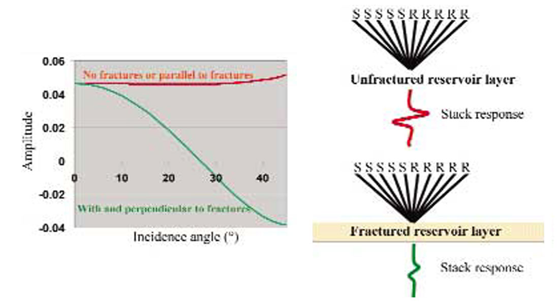
What is azimuthally varying AVO (amplitude variation with offset and azimuth; AVOA)? It is the change in amplitude gradient (i.e. amplitude variation with offset response) with azimuth from a reference direction, usually north. Figure 7 shows the amplitude response vs. incidence angle for a fractured carbonate. Parallel to the fractures the amplitude response is the same as if no fractures were present (the red curve). Perpendicular to the fractures (the green curve) the amplitude response is significantly different. Note the intercept or zero offset amplitude does not vary with azimuth. So, what does AVOA mean to an interpreter and how can the interpreter possibly use these properties of the pre-stack amplitudes?

First, AVOA does not just influence the pre-stack data. AVOA will carry over into the stacked amplitudes as well. When the AVO gradient is different in one azimuth than the perpendicular azimuth, the stack of these amplitudes over a wide offset range yields differing stack amplitudes (Figure 7). Therefore, in the simplest case, where 2-D lines intersect over a fractured reservoir section, the interpreter should not expect to have the same stack amplitudes. In the case of narrow azimuth 4-D acquired at differing azimuths, spatial amplitude differences between the two surveys may be due to spatial variations in the fracture density, rather than dynamic reservoir changes. Therefore, when evaluating the AVO in an anisotropic environment, the interpreter needs to be cognizant of the azimuth at which the AVO is measured. In one azimuth the AVO may exhibit a class II AVO; whereas, in the perpendicular azimuth, the reflecting horizon may exhibit no AVO or class I AVO.

In the interpretation of AVO from wide azimuth data, isotropic AVO analysis may be completely invalid because the AVO gradients are a mix of the differing azimuths. For wide azimuth data, the interpreter has two choices. Either solve for the azimuthally varying AVO solution, or only observe the AVO along one azimuth and realize that the AVO differences observed are only relative to that azimuth.

One other aspect of AVO from a fracture source is that the AVO gradient can cause intra-lithology reflections that may not be evident from acoustic impedance. Take for example a brittle shale interval within a thick interval of acoustically similar shale. The seismic synthetic from the sonic and density log may show no reflecting interface; whereas, a strong event may be present on the seismic data. In this example, a gamma ray or SP log is more likely to correlate with the seismic reflectivity than impedance from the sonic and density

Conclusion

The earth is anisotropic and P-wave anisotropy is often significant. Both the P-wave velocity field and amplitudes (pre-stack and post-stack) are influenced by the anisotropy. In addition, azimuthal anisotropy is an issue in narrow azimuth and 2-D data as well as wide azimuth 3-D. The interpreter, when aware of how the anisotropy manifests itself in seismic data, can incorporate these effects into the interpretation to evaluate risk. In addition, they may be able to extend the interpretation to address the source of the anisotropy.

Mostly this azimuthally varying anisotropy is attributed to fractures, which may not necessarily be macro fracturing related to reservoir permeability. Crampin has suggested micro-fracturing in the earth, which may not increase reservoir permeability, is prolific. This view is supported by our observations of P-wave azimuthal velocity anisotropy over large survey areas in various parts of the continental US. It should also be noted any alignment, whether depositional fabric or crystallographicly aligned cements filling fractures, may also cause the anisotropy. Therefore, we should not jump to the conclusion that what we observe in the anisotropy is always the open fractures.

Acknowledgements

The authors would like to thank Victor Vega (BP), Jon Huggins (Devon Energy), Chris Besler (Stone Energy) and Heloise Lynn (Lynn Inc.) for many useful discussions and comments on the issues relating to P-wave azimuthal anisotropy.