Interpreting Sand Channels from 3C-3D Seismic Inversions

Shear waves can provide vital lithologic information, especially in combination with traditional P-wave seismic data or when P-wave sections contain ambiguities. An example is the Lower Cretaceous Glauconite Channel play of southern Alberta, Canada. Here channels can be filled with sands and/or shales, each with similar P-wave impedances. However, from full-wave sonic logs, we find that S-wave impedance is higher in the sands than in the shales. The Blackfoot 3C-3D seismic survey was acquired over a channel area in hope of distinguishing the sand reservoir from shale. We should have a slight Vp decrease and significant Vs increase leading to a low Vp/Vs value. P-wave sources (dynamite) and 3-C geophones were used to record both P-P and P-S waves, We have used seismic inversion to transform the P-P and P-S components to P- and S-wave impedances. We then formed a volume estimate of Vp/Vs by dividing information from the two inversions, the objective being the discrimination of sands and shales. The higher frequency P-P inversion showed good detail within the channel and clarified the complicated seismic character at and above the dominant Mississippian unconformity. Agreement between the estimated Vp/Vs and available measurements from full-wave sonic logs was generally good. New prospective areas for exploration were identified from low Vp/Vs regions.

Introduction

The analysis of P-wave seismic reflection data can lead to ambiguous conclusions in certain exploration situations. Examples are the post-Mississippian Glauconite channels common to Central Alberta. Here, differentiation of prospective channel sands and non-productive shales is problematic due to the similarity in P-wave impedance of these two lithotypes Modelling (Miller et al., 1995) has shown that differentiation of sands and shales should be possible with the addition of shearwave information. This was the motivation behind the acquisition of the Blackfoot 3C-3D seismic program which was designed to acquire converted-wave (P-S) data in addition to the traditional P-P waves. Margrave et al, (1998) have used an isochron ratio approach for estimating Vp/Vs for these data. In this work, we seek a Vp/Vs estimate based on amplitudes. The analysis is facilitated by the transformation to impedance. This seismic inversion process presents the data as geologic layers rather then reflection edges. Seismic inversion transforms input seismic data to pseudo-impedance logs at each CMP. The algorithm employed here incorporates a seismic wavelet to compensate for both phase and amplitude effects. In the latter context, tuning is reduced and interpretability increased. To reduce non-uniqueness, geologic and geophysical constraints are applied during the inversion procedure. Inversion is done independently on each of the P-P and P-S data sets, creating two volumes of impedance. These are then used to form a third volume, an estimate of Vp/Vs. We then use the combination of these two types of information in the interpretation of Glauconite channel facies. In the project area, Cretaceous channels can be filled with both sand and shale. It has been observed (Potter et al., 1996) that the P-wave velocities of the sands is similar or slightly less than that of the shales, However, laboratory and l?g analysis has demonstrated that the rigidity and S-wave velocity of sand is greater than that for shale. This implies a decrease in Vp/Vs from shale to sand. In this experiment, we record and image arrivals from both P-P and P-S modes. Equating variations in the ratio of the P-P and P-S inversions with equivalent changes in Vp/Vs, we make 3-D estimates of lithology.

Geology

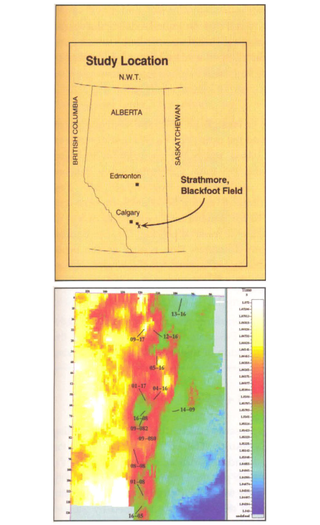
In the Blackfoot area, Lower Cretaceous sediments rest upon eroded Mississippian carbonates of the Pekisko Formation (Dufour et al., 1998). Above this unconformity is a detrital member of variable thickness which is itself overlain by ribbon and sheet Sunburst sands. Subsequently, marine transgressions deposited the brackish shales, limestones and quartz sands and silts of the Ostracod. The Glauconite in Southern Alberta consist of shales and quartz sands of lacustrian and channel origin, Three phases of channel development have been identified during this period with the possibility of different degrees of incision and different quality of sands deposited. Porosities of up to 18% have been observed. The primary target is oil with gas also possible in the more shallow sands. Figure 1 shows the project area and the interpreted time structure of the Glauconite horizon.

Methodology

3-D geologic model

The outcome of the seismic inversion implemented in this paper is the trans formation of seismic reflection data to pseudo-impedance logs at each CMP. But first, a 3-D geologic model of the project area is created. The uses to which we put the model are two-fold. It is necessary to apply geophysical constraints to the inversion of the seismic reflection data. The constraints, which remove much of the non-uniqueness in the solution, are interpolated through the project at each CMP along the layers defined within the model. In this way, the constraints become attached to particular facies and vary appropriately with structure. Additionally, the raw inversion solution will be poorly constrained at frequencies below the seismic band. We can replace these frequencies with more reliable information from the geologic model. The low-frequency impedances are obtained by populating the model with P-wave and S-wave sonic logs along with bulk density information.

Wavelet analysis and seismic inversion

Wavelet analysis is completed by computing a filter which best shapes the well log reflection coefficients to the input seismic at the well locations. The phase of the seismic data, which may vary with frequency is found from the inverse of this filter. This wavelet, with amplitude representative of the seismic data, is input directly into the inversion algorithm. Two wavelets must be determined corresponding to the P-P and P-S wave data sets.

In seismic inversion, the following question (but in mathematical terms) is asked, "For each seismogram at a particular CMP, which reflection coefficient series, when convolved with the wavelet produces a synthetic which replicates the input reflection data?" The solution is found by minimizing a combination o f L1 and L2 norms , subject to a set of constraints (Debeye and Van Riel, 1990). The most important constraint limits the solution space to a " fairway" of allowed impedances defined a teach horizon. The constraints are defined loosely enough to admit the possibility of all expected geological results.

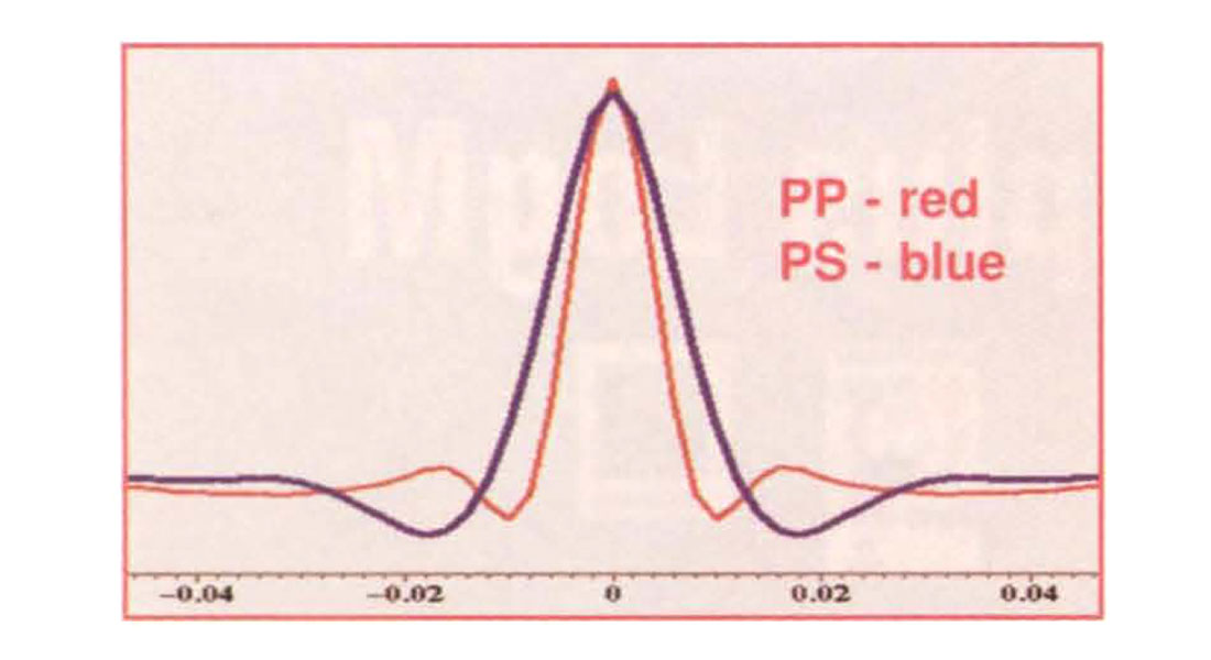
No a priory knowledge of impedances beyond the solution space defined by the fairway constraints is provided at the well locations. This makes comparison of the filtered impedance logs and inversion impedances at the well locations a natural quality control. The inversion is in fact performed iteratively when the input horizons from the seismic reflection interpretation are approximate. The constraints are first set loosely and an initial inversion is created to better define the geologic layers. The interpretations of the horizons are then improved from the inversion and the constraints tightened around them. Finally, the inversion is re-run using the tighter constraints. All horizons shown in this paper are the results of reinterpretations from the inversions. Each of the pop and P-S stacked data sets are inverted separately using the appropriate wavelet. The extracted wavelets are shown in Figure 2.

As discussed above, the lowest frequencies from the raw inversion procedure can be replaced since they are ill-constrained by the seismic data. When the horizons are known accurately and there is sufficient well information, a detailed model can be built and in turn used to provide an equally detailed geologic setting in which to place the inverted seismic-band information. Alternately, a single well or impedance function could be used to define a simple, reasonable model.

Estimation of Vp/Vs

While the results of inversion are P-P and P-S impedance cubes, we seek to estimate the ratio, Vp/Vs. We first describe an estimation procedure based upon the assumption of equal resolution of the pop and P-S data. Converted-wave data are often pre-processed assuming a Vp/Vs of 2.0. This approximately aligns the P-P and P-S sections in time and facilitates tying them. To compute accurate estimates of Vp/Vs from the inversion data, the tie must be precise. This can be done most easily in the depth domain. Fine tuning of the depth conversion velocity functions can be used to achieve an optimum tie. This computation yields a Vp/Vs value at each time sample within the region of interest.

For the purposes of this work however, we recognize that the frequency content of the P-S data is less than that of the corresponding P-P in the region of interest. We begin by making the identification:

In equation 1, δ^P-P represents effects due to P-wave stacking for which we do not account. The δ^P-S term represents the equivalent S-wave effects and in addition, compensation for the approximation, Vs ≈ Vps. In principle, the offset P-S reflectivity values should be converted to a zero-offset normalized velocity change. A procedure to do this has been described by Stewart (1991). Here, we have chosen to compute ratios of the P-P and P-S inversions, applying a spatially in variant calibration derived by comparing to observed values of Vp/Vs at the wells. Our assumption is that the converted waves provide additional information about lithology which is manifested in this quantity. The measurement of Vp/Vs is made from observed data by computing the ratio of the two inversions. Each inversion is the sum of low and high frequency components. We write,

We refer to the high- frequency components in equation 2 as relative inversions, containing in formation transmitted only by the seismic reflection data. In this work, we assume that the low-frequency components are constant across the project area. As shown below, the vertical resolution of Zps is limited and in fact, only one estimate of channel impedance has been made at each (Mr. Then, rather than divide a P-wave impedance cube by a P-S impedance cube, we divide by a P-S impedance horizon representing the average P-S impedance at each CMP. Or:

We plan further work to evaluate the accuracy of the above approximations. However, our immediate goal is to evaluate the information content of the seismic (high) frequency component of the inversion. Equation (3) admits that possibility. Using the layers defined by the geologic model, maps can be made of the average Vp/Vs for thin layers conformable with key horizons.

Data

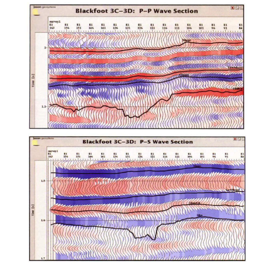
The Blackfoot 3C-3D seismic survey was acquired near Strathmore, Alberta, Canada in 1995 (Stewart et al., 1995), The Glauconite channel is located in the north-west section of the survey. It is this subset consisting of 115 lines and 83 CMP's that is analyzed here. The bin size is 30 x 30 m and offsets ranged from 300 to 1700 m. Approximate alignment of the P-P and S-S sections was done during processing. There are 11 wells within the project area, as shown in Figure 1. Dipole sonics were available for five of these. Most wells are somewhat deviated. An interpretation of the reflection seismic was done by CREWES personnel at the University of Calgary and was used to construct an initial model. Figure 3 shows examples from the P-P and P-S data sets. There is less frequency content in the converted-wave data and as will be demonstrated below, an attendant reduction in resolution in the inversion.

Results

Geologic Model

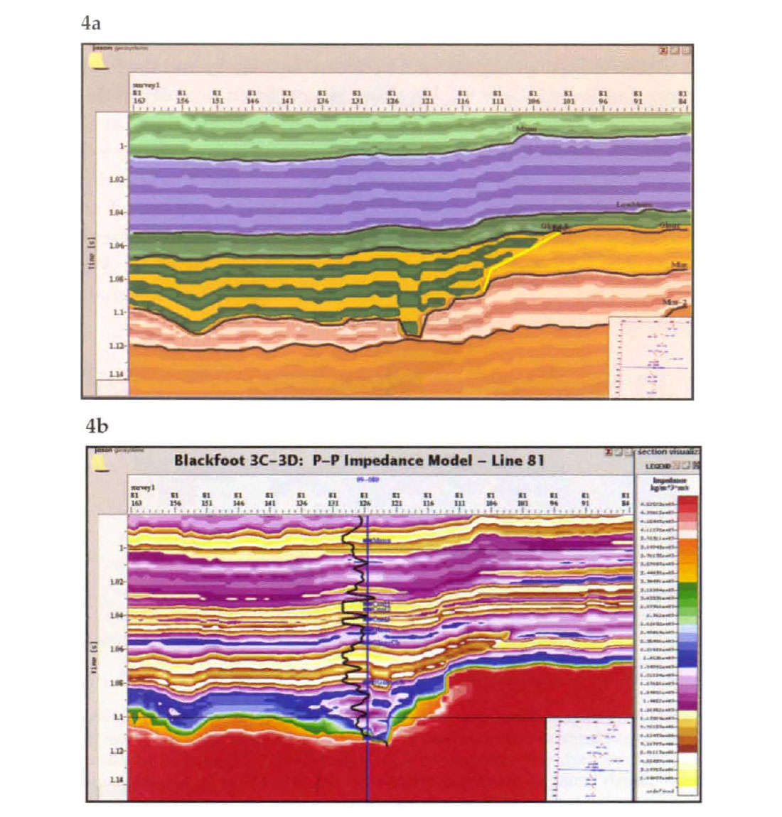
Geologic models with a 2 ms sample interval were constructed from the interpreted horizons and a framework table describing the arrangement of the layers. A section through the PP model structure is shown in Figure 4 (left panel). The broad colours are meant to indicate the laver boundaries. The structure of the finer banding internal to each layer is indicative of the stratigraphy. Figure 4 (right panel) is the same section through the final Pop impedance model. Lateral variations in impedance arise from both structural and stratigraphic effects. At CMP's where no log is present, nearby logs were stretched or squeezed on a layer-by-layer basis to account for structure and then subjected to a weighted average to arrive at the model impedance. A simple distance-weighted average sufficed although the weights could have been set arbitrarily as required.

Constrained Sparse Spike Inversion

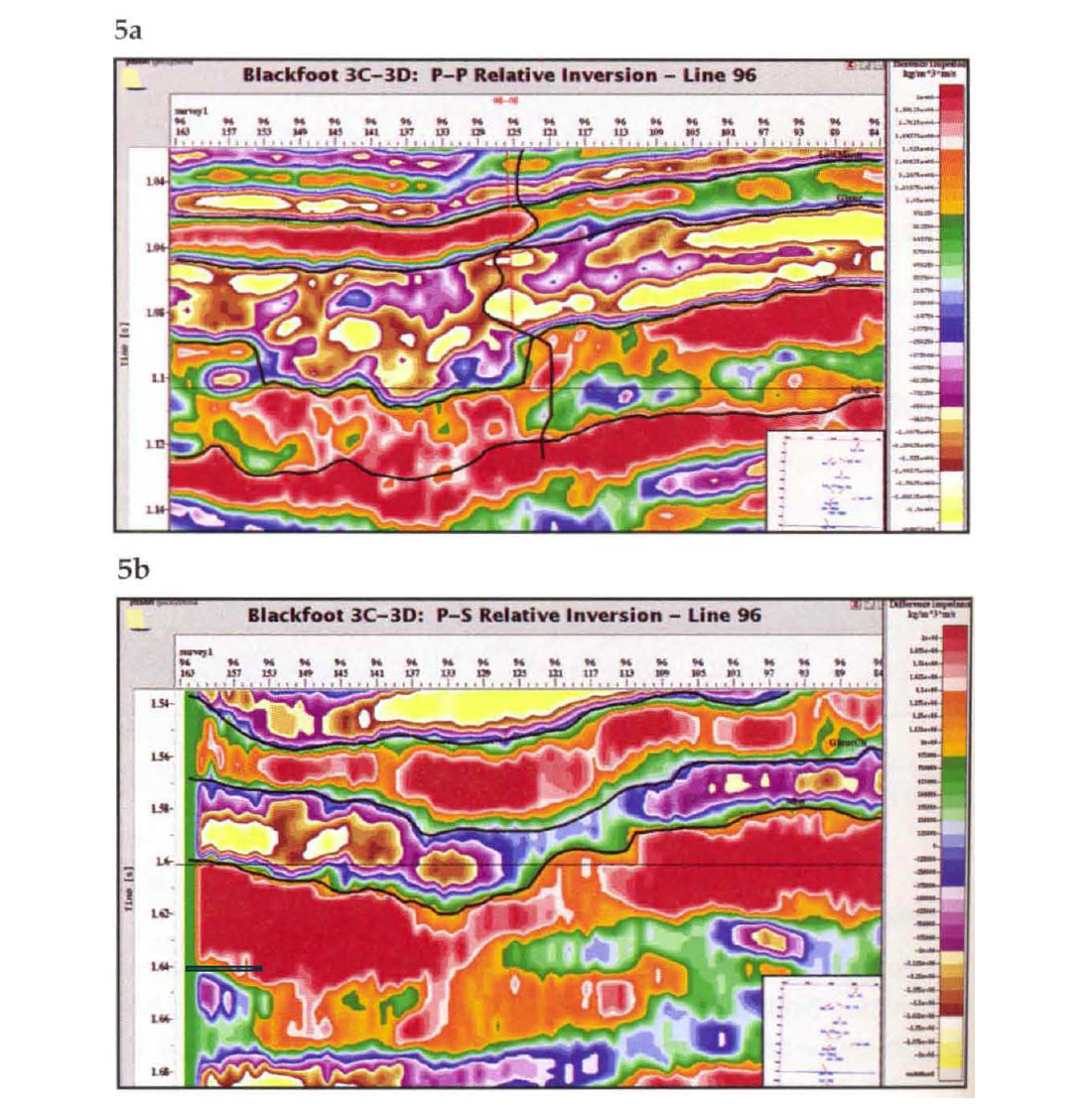
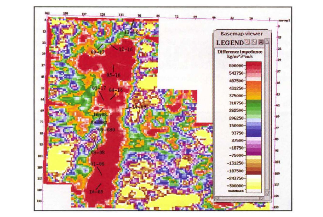
Wavelet analysis was done separately for the P-P and P-S data. In each case, the seismic data were matched to the appropriate impedance logs at the wells and wavelets estimated. The P-P and P-S wavelets were close to zero phase. The inversion methodology described above was used to compute both Pop and P-S inversions. The horizons were then re-interpreted from the initial inversions, after which the inversions were re-run. Line 96 from the pop and P-S relative inversion is shown in Figure 5. In the P-P section, considerable detail is evident around and within the channel. The somewhat confusing character of the Mississippian in the seismic is seen to be the manifestation of a layer of intermediate impedance just above. We interpret this to be a detrital facies. Low impedances in and about the channel could be sand or shale. The character of the channel facies in the inversion is suggestive of layering with different episodes of deposition and is consistent with the three-valley model of Dufour et al ., (1998). The frequency content in the P-S data is obviously less. Here, the channel appears as almost a single entity. We have chosen to make use of only the average P-S inversion value at each CMP. This parameter is mapped in Figure 6. Although all of the velocities in the channel are low, dark red represents the relatively highest of these. Notwithstanding the lack of resolution, the channel is well imaged in the figure and lateral variations in the P-S impedance appear to be reasonable (see discussion below). There is what could be interpreted as a crevasse splay feature to the north end of the channel.

Estimation of Vp/Vs

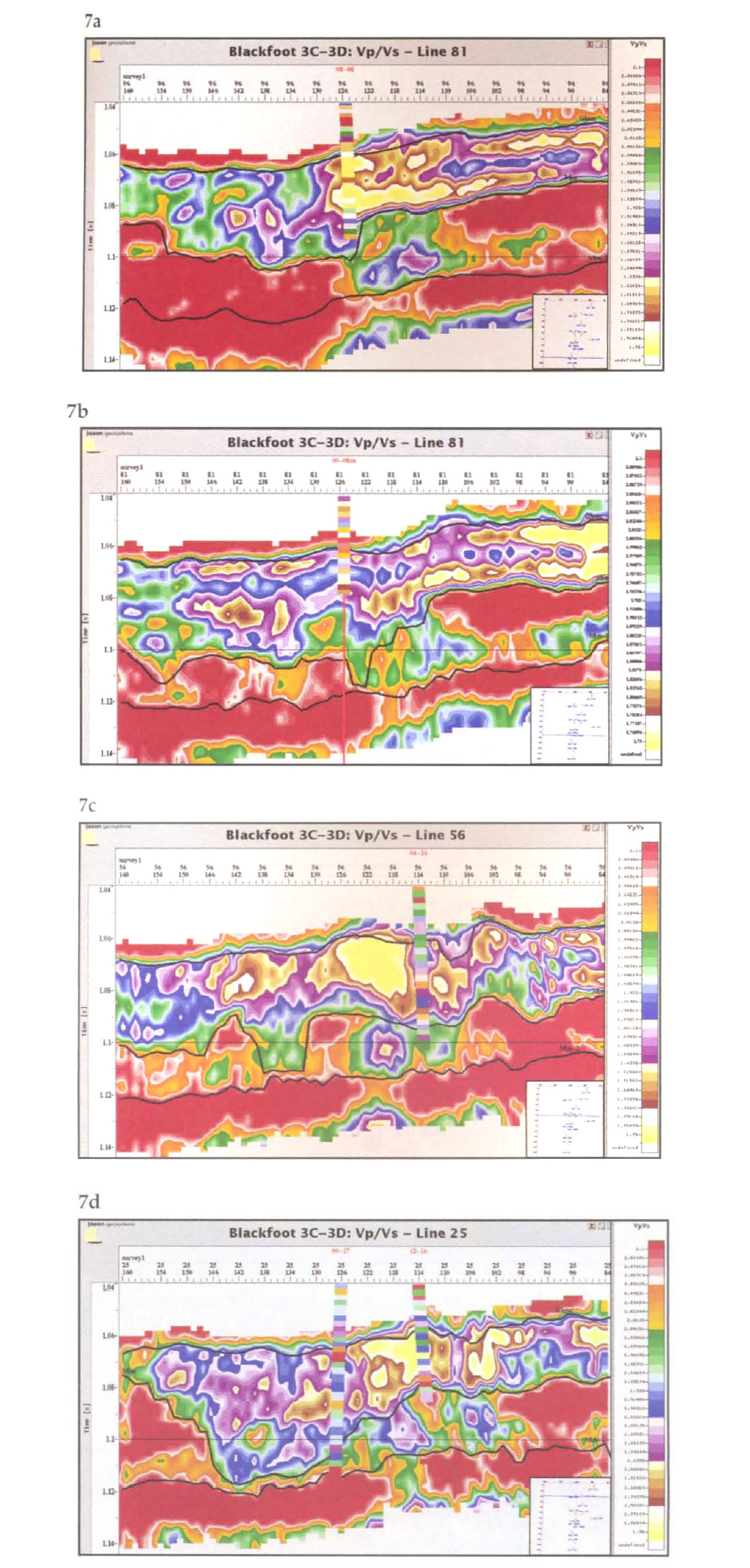
The P-P impedance volume and the P-S impedance map were used to compute a Vp/Vs volume following the methodology described above. We expect a low Vp/Vs ratio to be indicative of sand. Arbitrary sections were extracted near the wells and are shown in the Figures 7 below, with the Vp/Vs curves from the wells superimposed. Figure 7a is an example of good fully developed porosity in both an upper and lower sand.

There is excellent agreement between the 8-8 logs and the field data. In Figure 7b, the 9-8 log showed significant porosity in the lower sand only. The estimate of Vp/Vs reflects this. Logs at 46 showed little porosity (Figure 7c) and the facies was interpreted as a shale plug. The Vp/Vs estimate indicates potential nearby porosity development. In Figure 7d, well 9-17 is described as " regional" while 12-16 encountered some deep sand. Agreement is good at 9-17 and poorest in the shallow channel at 12-16. We note that the 12-16 location is situated in a region of poor signal-to-noise ratio in the P-S reflection data.

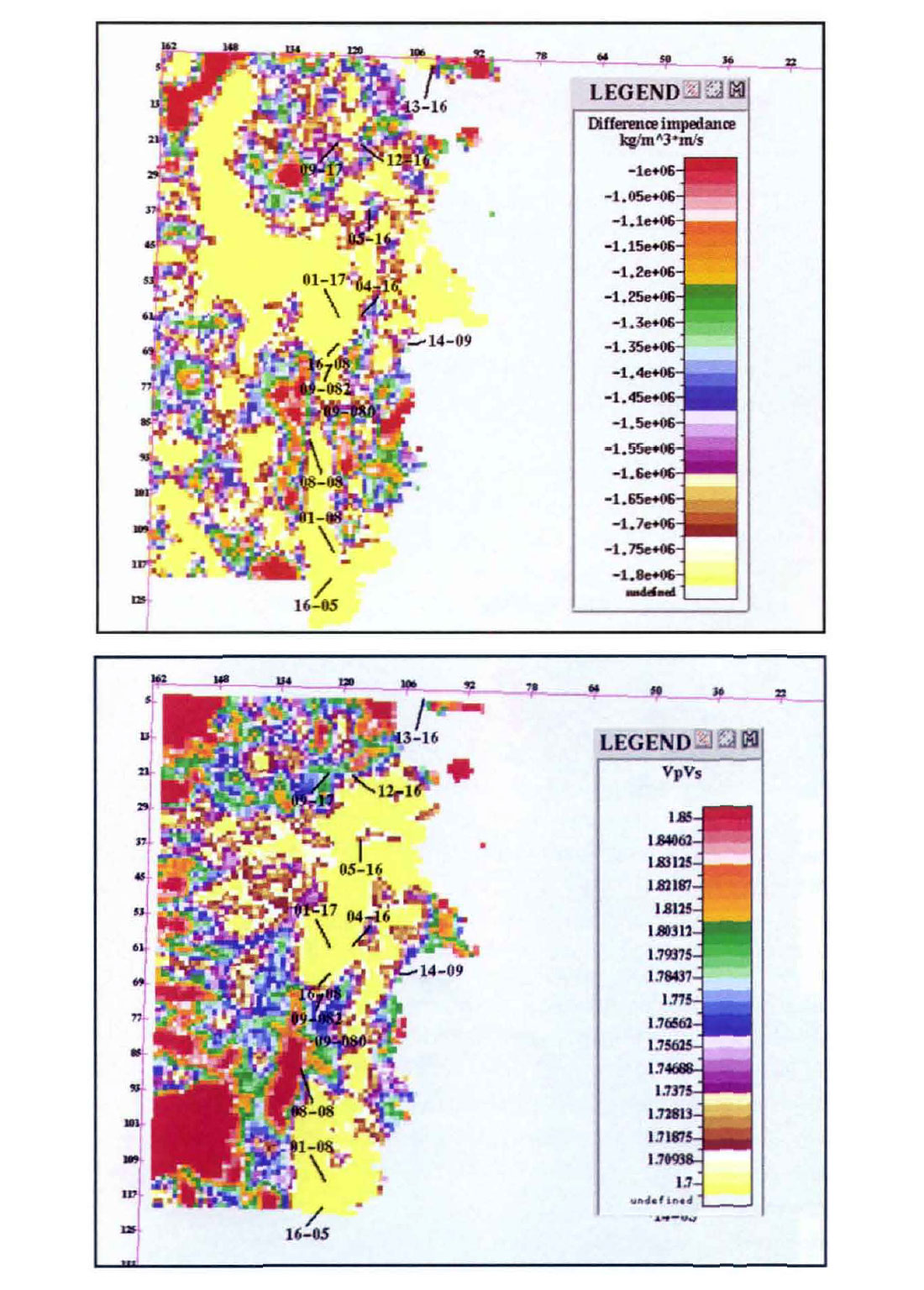
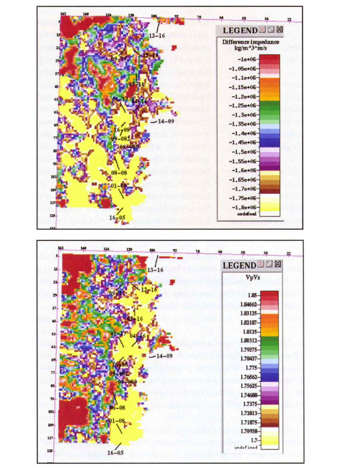
We have also mapped both the lateral variations of P-P impedance and of Vp/Vs. Recognizing the increased resolution in the P-P data, smaller time intervals were chosen for mapping.

Shallow, middle and deep channel facies were identified based on changes in pop impedance distribution. The results are shown in Figures 8 to 10 with the maps of pop impedance on the left and Vp/Vs on the right. Each pair of adjacent maps was derived from the same time interval. Yellow represents the lowest Pop impedance and also the lowest Vp/Vs. In these figures, the channel edge interpreted on the P-P inversion has been used to re-build the geologic model and limit the map to the channel facies. Clearly different depositional regimes are in operation here. The low impedances in the P-P maps can represent either sand or shale. In the middle layer there is a low impedance trend to the north located to the west of the main area of exploration interest. It is apparently shale-filled as it is not represented on the corresponding Vp/Vs map.

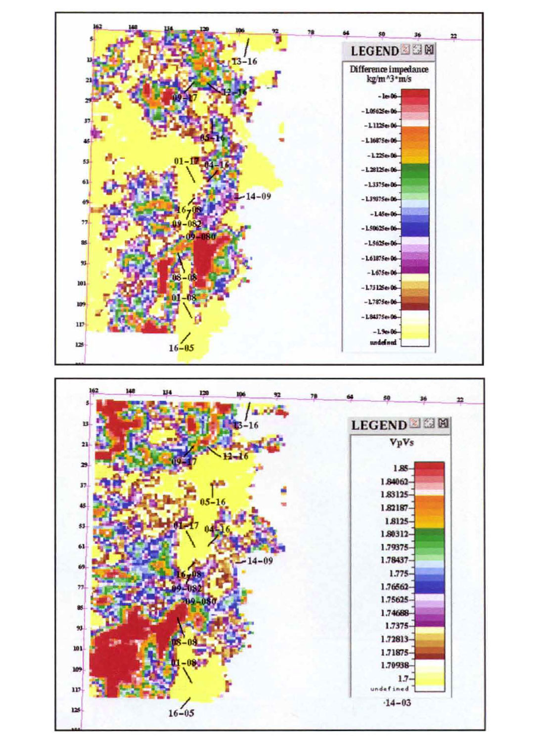
There are indications of new prospective areas. Good Vp/Vs is indicated to the south of 9-17 in the P-S "crevasse splay" centred at line 3-1 and CMP 135. There is also very low Vp/Vs immediately to the west of 4-16, the well in which the shale plug was encountered. The Vp /Vs maps also show that 8-8 is just on the northern edge of another region of low Vp/Vs. Consideration to drilling locations to the south of 8-8 could also be given.

Conclusions

This paper has developed seismic inversion techniques that can be used to improve the imaging and interpretability of post Mississippian channel facies. P-P inversions can image and map regions of anomalously low impedance which can be representative of either sands or shales. Notwithstanding the sand-shale ambiguity, good definition of lithology is possible. In the example presented here, the deposition and composition of post-Mississippian sediments was clarified. The P-S inversion has been demonstrated to be a "sand detector" with good lateral but limited vertical resolution. Vp/Vs volumes can be created from 3C-3D seismic reflection data and mapped to discriminate between sand and shale-prone regions. Agreement with full wave sonics was generally good.

Acknowledgements

The authors gratefully acknowledge the assistance of CREWES staff at the University of Calgary and also acknowledge support of the CREWES Project sponsors. We also acknowledge the support of Pan Canadian Petroleum, owner and operator of the Blackfoot field.