Interpolation, PSTM, & AVO for Viking and Nisku Targets in West Central Alberta

Summary

West Central Alberta has a thick stratigraphic section (up to 5000m) with multiple exploration and development targets in conventional clastic, carbonate, tight sand, and shale reservoirs. Compressional and extensional structural features are common throughout this large region, particularly further west. The area has extensive 3D seismic coverage, but that coverage typically has coarse source and receiver line spacing. AVO attributes have superior exploration and development utility for many of the targets as compared to conventional stacked data, but the use of AVO on any of these zones are challenged by the difficulty in extracting accurate AVO results. One of the variables that adversely affect the accuracy of the AVO extractions is the coarseness of the 3D seismic geometry. This coarse 3D geometry causes migration artifacts on our migrated gathers that arise due to the insufficient sampling of the seismic wavefield. This issue led us to use a 5D interpolation prior to migration to minimize these artifacts. We chose two current exploration and development targets to illustrate the effectiveness of this new method of AVO processing: the Viking, and the Nisku.

The Viking is a prolific zone that is deep, structured, and very thin relative to tuning thickness. We attempted to exploit the AVO response of this gas-charged zone on migrated gathers to obtain a more accurate estimate of Phi-H than we could achieve with conventional amplitude mapping. In order to evaluate the performance of the new interpolation workflow, we performed our AVO analysis with a number of other relevant and established competing techniques. This interpolation migration flow was the most effective flow relative to other methods tried on this data, and represents an important new paradigm for land AVO analysis. This assertion is validated by 29 well ties and the resultant maps which are consistent with the structural erosional model of the Viking.

The Nisku carbonate play was also subjected to our new interpolation migration method. Evaluating the performance of the new paradigm is aided in this case by the fact that one of the 3D seismic surveys in the area has been the subject of a previously published AVO case study on the Nisku. As such, we have an excellent control study to compare against our new method. We generate AVO Inversion results that behave in a more physically reasonable manner in cross plot space, tie the wells better, and produce cleaner, more geologically consistent maps than the previous study was able to produce.

By illustrating our new interpolation migration method of AVO processing on these two very different targets, we demonstrate the general importance of stabilizing prestack migration with this kind of support on structured, coarse 3D seismic surveys. These examples offer some insight into the future direction of other, related methods of analysis such as Azimuthal AVO (AVAz), whose sampling is much worse and could be expected to benefit from this kind of imaging support.

Introduction: interpretive challenges

Seismic processing and interpretation is at once a scientific, and a hopeful endeavour. The presence of noise, inadequacies of the acquisition parameters, interpretive or physical non-uniqueness within the resolution at hand, and sometimes even the lack of sufficient geologic sampling to adequately understand all aspects of the problem, all serve to add uncertainty to our ability to confidently interpret seismic data. Our approach must always be as scientific as the shortcomings of our data allow, and constantly engage in the pursuit of improving our method against these same limitations. Whenever we attempt a new technology to attack or mitigate against the ill-posed nature of our interpretive pursuit, there is a certain element of hope that these efforts can enable us to do better.

The interpretive examples shown in this paper are somewhat disparate: the thin gas-charged clastic Viking zone and the Nisku reef of West Central Alberta. These zones make interesting representatives of a large suite of similar or related interpretive problems within the Western Canadian Sedimentary Basin. The Viking is very thin, but is over pressured and gas filled. The Nisku is very deep, and while thicker, has a lithologic uniqueness problem with some of its basinal equivalents. Both are set in a structural regime and are covered by 3D seismic data. In forming the geophysical element of a strategy around how to explore and develop these zones, we first considered the various seismic attributes that we might extract from the data.

There have been many recent efforts to categorize the various attributes in order to make this exercise easier.

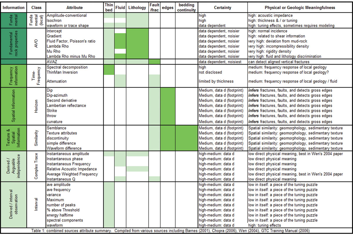
Table 1 represents a classification scheme inspired by and heavily borrowed from the work of Barnes (2001), Chambers (2002), Wen (2004), and Chopra (2006). The classification scheme attempts to break the attributes into types of information, certainty of their information, kind of geophysical problem they address, and physical meaningfulness. The color overlay indicates qualitatively the level of discrimination the attribute might be able to provide. A darker green color indicates a higher degree of discrimination. It is clear that depending on the particular exploration problems at hand, the useful or important attributes will change. It is also clear, however, that certain of these attributes contain more fundamental and broadly useful information than the others. The most fundamental attributes are, in fact, the rock property type attributes that are estimated through AVO analysis. This makes sense when we consider that the stacked trace is a complex mixture of contributions from the AVO attributes. One might argue that shape and texture attributes are also fundamental in some ways, but the AVO attributes attempt to represent the rock properties directly, and are there f o re the most universally useful elements of information that may be estimated from seismic data. The well known problem with these attributes is that their certainty is poor. One might argue that some amount of effort towards AVO analysis should always be employed on seismic data, except for the difficult, ubiquitous, problem of the difficulty in accurately extracting this data. This uncertainty almost always forces us to retreat to using the more robust stacked trace as our fundamental unit to extract the other attributes from, even though we know that the AVO attributes would make more physical sense as the starting point. If having better AVO attributes would help us on our interpretive endeavours generally, then it makes sense to continue to improve our methods of AVO analysis. Much current research is being directed into this worthwhile pursuit, with this paper directly concerned with improving AVO analysis through a method of interpolation.

Interpolation is useful and relevant because most AVO-sensitive plays need to be accurately imaged in space as well as time, requiring prestack migration. The more structurally complex the area, the more important this consideration is, although even for stratigraphic plays migration is important to collapse the Fresnel zone. Despite these considerations it has been questionable whether land seismic data processed specifically for AVO analysis should be prestack migrated due to the migration artefacts introduced as a result of the sparse acquisition typical of land acquisition. Land 3D seismic surveys are commonly shot with coarse, irregular geometries. This lack of regularity causes migration artefacts on the imaged gathers which can be a serious contributor to the overall noise level. By interpolating the data in an AVO-preserving manner prior to migration, we mitigate or reduce these artefacts with minimal harm to the sharpness of the image. Other methods of noise reduction commonly require mixing, averaging, or stacking after imaging, which has the consequence of smearing structural information.

We will illustrate and support these statements in our paper through our discussion of the Viking and the Nisku exploration and development problems. In the Viking we will employ a rigorous method of comparing the usefulness of the interpolation method as compared to the older, established ways of handling the data. Our comparison is less rigorous in the Nisku, but we will utilize the available well control for validation purposes and investigate other indications and effects of noise on the results. We will also discuss issues of quality controlling the interpolation method, and address future work.

It should be pointed out that much of the following work is taken directly from Hunt et al. (2008) and Reynolds et al. (2008), of which this paper is a compilation.

The Viking challenge

Viking Formation reservoirs in West Central Alberta represent attractive exploration targets. Reservoirs are comprised of shoreface sandstone assemblages that often retain 12-14 percent porosity over 0 to 7 meters thickness, and occur at depths greater than 2800m. The sandstones have low permeabilities (< 1 mD) but are commonly overpressured and gas-bearing with typical recoverable resource of 8 Bcf and 80,000 bbls condensate per section. The structural setting for the area includes both extensional and compressional tectonic elements.

Figure 1 is a schematic cross section of two wells within the 3D survey. These wells were selected for the modeling work as they had full wireline log suites including shear and compressional sonic and core data. The section is hung on the Base Fish Scales (BFS) and shows two basin-wide transgressive events labeled VE3 and VE4 (after Boreen and Walker, 1991).

The preserved porosity in Well A is associated with the upper shoreface deposits below the VE3 surface.

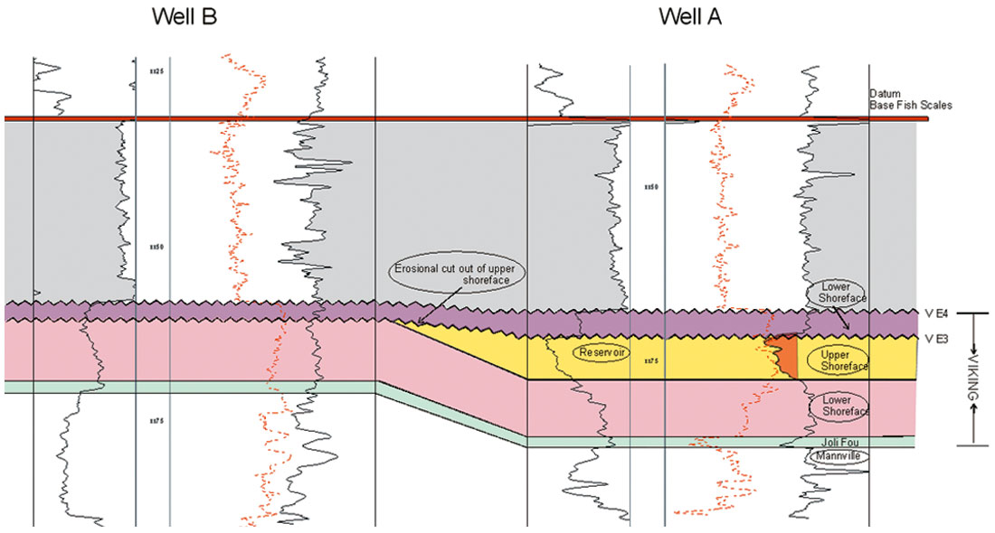
In Well B the VE3 surface is underlain by tight lower shoreface and basinal deposits with no reservoir quality. Tectonism during Viking time may have caused reactivation of basement-rooted faults which created an irregular sea floor topography that was differentially eroded during basin-wide transgressive events resulting in the complex aerial distribution of preserved porosity. In general, porous and permeable progradational shore face deposits are preserved in structural lows.

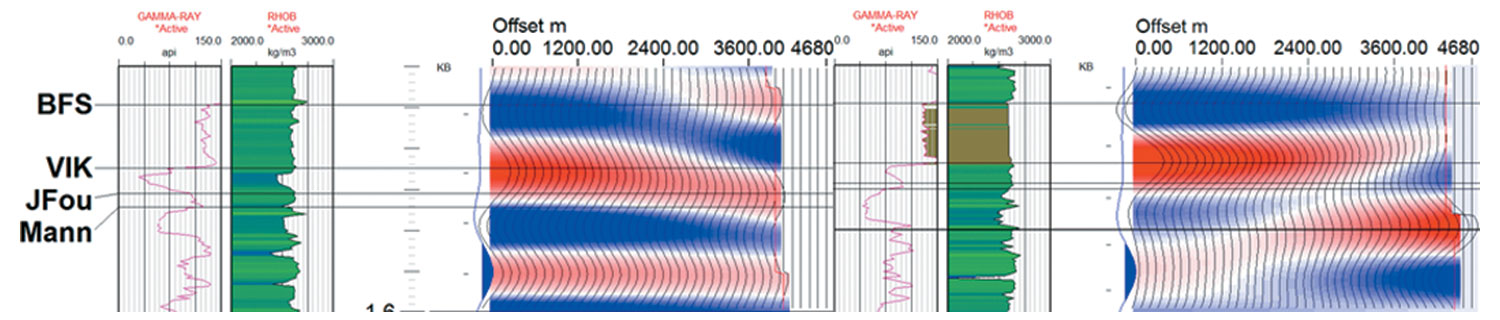
Despite the coverage of 3D seismic, accurate reservoir prediction is very challenging. The productive reservoir, which may be entirely or partially eroded, is never greater than 1/15 of a wavelength in thickness. These variables contribute to a poor correlation between seismic amplitude and measures of porosity thickness. Recalling Figure 1, the Viking can be described as a more competent material sitting under a less competent halfspace (the BFS zone). Thus the Viking is a peak on a zero phase stacked section. When porous and gas-charged, a well resolved Viking zone may have a Type IIa AVO response, where the weak peak goes towards smaller amplitudes with increasing offset. Log data from Well A and B illustrate this response with the good quality reservoir in Well A versus the absent reservoir in Well B.

This response suggests that an advantage may lie with the utilization of this contrasting AVO effect. The structural setting demanded the use of PSTM gathers for the analysis. Unfortunately, the 3D coverage in the area has coarse source and receiver line geometries, which give rise to gross irregularities in the offset and azimuthal distribution of the data. Upon PSTM, these irregularities cause distortions which adversely affect the AVO analysis.

The Nisku challenge

In 2005 Pelletier and Gunderson published a thoughtful, petrophysically driven, work on AVO Inversion for a Nisku target in the Brazeau area. They attempted to discriminate low impedance basinal Cynthia shales from porous Nisku Reefs using AVO inversion on a 3D seismic survey. Their AVO Inversion techniques followed a rationale derived from petrophysical analysis of Lamé’s parameters from wireline data in the area. The work appeared to be successful in that it seemed to identify 4 known reefal wells, and also identified 2 new prospects. There were no basinal wells available on the 3D survey at that time. We use the modifier “appeared” simply because the amount of drilling control remained statistically insufficient for greater confidence. In the time since that paper was published, 10 new wells have become available, and several new technologies have been adapted to improve the veracity of AVO Inversion products. Of particular interest is the fact that Pelletier and Gunderson’s analysis was performed on CDP gathers rather than image gathers. Since then, new 5D amplitude-preserving interpolation algorithms have become available. These interpolation algorithms can minimize migration artefacts allowing us to improve our AVO estimates. We compare the AVO analysis based on the original and reprocessed flow including interpolation and PSTM. We will utilize the new drilling data to help us objectively quantify the improvements to be gained by using our interpolation migration method of AVO analysis, and discuss whether these new improvements add enough value to warrant reprocessing of even recently analyzed data.

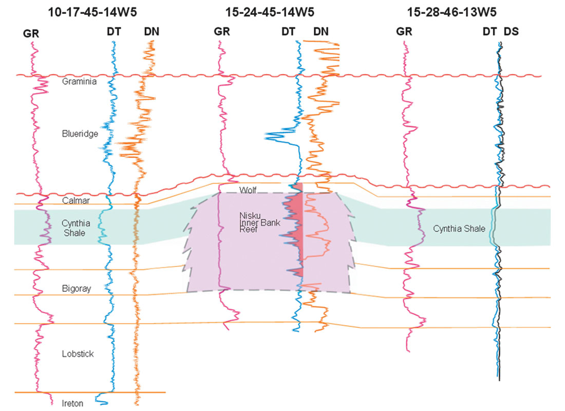
Exploration for gas-bearing Nisku reefs in the Brazeau area represents a classic challenge for seismic lithologic prediction. The basinal Cynthia member is stratigraphically equivalent to the Nisku reefal carbonates. When the Cynthia member is sufficiently argillaceous, it has a strong gamma ray response, a low rigidity, and may appear very similar to the porous Nisku reef on conventional stacked seismic. In this case, our challenge would be the separation of higher rigidity, lower Lambda*Rho reef from lower rigidity shale – a classic carbonate AVO Inversion problem. The Cynthia member can also be more calcareous as well, which would re p resent a different problem seismically. In such a case, wireline data would see less of gamma ray response, and the rigidity would be higher – potentially higher than the reefal facies. Figure 3 represents these facies differences as measured by wireline logs.

Pelletier and Gunderson (2005) focussed more on the calcareous element of the basinal response. With further drilling since their publication, we have been able to sample the potential lithologic outcomes more completely, and can address a wider range of reefal and basinal possibilities. Table 2 represents the rock properties we would expect from the key end members we wish to represent.

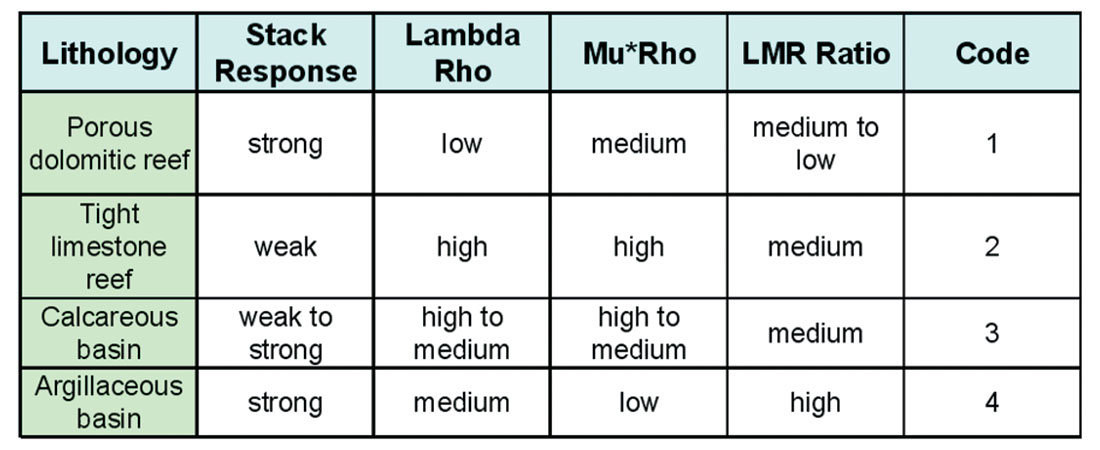
Figure 4a is a Lambda*Rho versus Mu*Rho cross plot from Pelletier and Gunderson (2005). As stated earlier, critical sampling of the argillaceous basin was not available at the time of that publication, and the facies was therefore not fully re p resented. In Figure 4b we illustrate a Lambda*Rho versus Mu*Rho cross plot calculated from currently available wireline logs on or near the 3D. In this case, we used data points from 3 reefal wells and an argillaceous basinal well that discriminates the lower rigidity we expect from that facies. The augmented petrophysical sampling that is currently available should improve our ability to discriminate facies in cross plot spaces estimated from the 3D seismic.

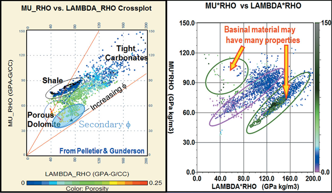
It is clear that accurate estimates of Mu*Rho are key in order to carry out the necessary discrimination. Lambda* Rho is also important, but is subject to smaller experimental error than the estimate of Mu*Rho. This is a consequence of the fact that Mu*Rho is calculated solely from the S-impedance reflectivity (Goodway, 2001) which has larger uncertainty in the presense of noise than the P-impedance reflectivity (Downton and Lines, 2001). By interpolating and then prestack migrating the seismic data, the signal-to-noise level is improved. This is a result of the better sampling of the wavefield prior to the migration, resulting in less migration artifacts and noise. Pelletier and Gunderson’s work was carried out on CDP gathers at a time when this kind of interpolation migration flow was not available. We will evaluate how much of an improvement comes from using the new method over the old by comparing the original Pelletier and Gunderson AVO attributes to the same attributes extracted using our new method. Validation is carried out using the current, improved, well control in the area.

Theory

Fractional elastic parameters such as the compressional (R_p) and shear reflectivity (R_s) may be estimated from the prestack seismic data by AVO Inversion such as the two-term Gidlow et al. (1992) equation R(θ)=R_p sec² θ – 8R_s γ² sin² θ, (where θ is the average angle of incidence and γ is the average S-wave / P-wave velocity ratio. There exists a wide variety of AVO attributes that could have been used for mapping and validation in this paper. For the Viking zone, we chose a very simple parameter, the damped R_p to R_s ratio, while we chose Goodway’s (2001) Lamé parameters for the Nisku zone. Unfortunately, all of these parameters are notoriously difficult to estimate with the fidelity and resolution to be useful on many stratigraphic prospects. Yi, Downton, and Xu (2007) describe the crucial challenges involved in successfully estimating the elastic parameters. Those challenges include the need to obtain migrated gathers that have sufficient resolution and high S/N ratios. In these examples, the structural deformation appears to be significant enough to require that AVO be performed on PSTM gathers. The nominal source and receiver line spacing of this 3D survey is 600m, and the data is noisy and bandlimited to about 55Hz. This acquisition geometry was not sampled sufficiently fine enough so that the wavefield would constructively and destructively interfere to image all the reflectors with a good S/N ratio.

To address this issue a 5D interpolation method (Trad, 2007) based on Minimum Weighted Norm Interpolation (MWNI) (Liu and Sacchi, 2004) was employed to regularize the data prior to migration. The goal of this interpolator is to detect poorly sampled coherent information and make it available for other processing techniques like migration. The 5D interpolation is performed by solving a large inverse problem in the inline-crossline-offset azimuth and frequency domain. In this case the desired model is a super-sampled seismic dataset, the data is the original seismic dataset, and the linear model is the sampling operator. The resultant super-sampled seismic data contains data for every possible inline, crossline, offset, and azimuth combination. In practice this creates so much data that it becomes impossible to deal with, so the algorithm only outputs a representative subset of this. In this case we output twice as many shot and receiver lines as the original geometry, thus preserving the original geometry and data as a subset of the new volume. As the original data are preserved, it is easy to verify that the original AVO trend is preserved. Further, the minimum norm constraint applied in the spatial frequency domain tends to ensure that the amplitude changes slowly in all four spatial dimensions including offset and azimuth while honouring the original data.

The high dimensional nature of this method permits the use of information from different spatial directions simultaneously and hence to infill geometries with very sparse sampling, beyond what is possible when working in a lower dimensional space. However, this capability should not be abused, there f o re traces created at a large distance from the acquired data are automatically discarded. This distance is measured in the five dimensional space where the interpolation takes place. Also 5D windows which do not have a re q u i red minimum number of live traces are not interpolated. Other typical quality control techniques are limited offset/azimuth stacks, which may be viewed as timeslices in addition to inline and crossline directions, and prestack gather inspection to check for amplitude and traveltime consistency.

Gather comparisons

Let us compare the effectiveness of the new interpolation method on individual gathers first for the Viking, and secondly, for the Nisku zones.

Figure 5 (a, b, c, d) shows a comparison of the original data at the Viking zone’s well locations A & B versus the interpolated data at the same locations. The AVO trend of the data has been preserved and is similar to the models shown in Figure 2. Similarly, Figure 5 (e, f, g, h) compares the prestack migrated (uninterpolated) data to the PSTM gathers after interpolation. For all the cases the interpolated results have a superior S/N ratio than the non-interpolated gathers. This is partly due to the higher fold and, in the case of the interpolated PSTM gathers, better sampling of the wavefield prior to the migration resulting in less migration noise.

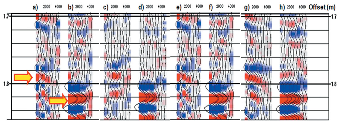
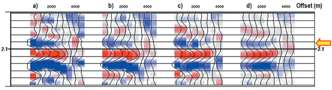
Figure 6 is an Ostrander gather taken at an argillaceous basinal well location. As Pelletier and Gunderson used super-binned CDP gathers for their AVO analysis, we illustrate a CDP gather in Figure 6a versus a super-binned CDP gather in Figure 6b. Our new method is illustrated by comparison with a PSTM gather in Figure 6c and the interpolated PSTM we advocate in Figure 6d. It is clear that the interpolated results have a superior S/N ratio. This is due to the higher fold in the non-migrated examples. In the case of the interpolated PSTM gathers, better sampling of the wavefield results in less migration noise. Note that all the gathers shown have been partially offset-stacked with the same offset binning so that the figures may be easily compared.

Viking test case: 3D seismic with significant well control

The 3D that we used for this test had some 29 Viking penetrations. Since the primary geologic goal was to predict Phi-H in any new prospective well, we loaded the Phi-H value as a top into each well on the 3D. We then extracted our R_p/R_s ratio attribute at each well point and plotted the attribute versus Phi- H. To quantify any improvements that our new method might yield, we created several versions of the data. Each version was processed identically to the others- except for the noted change (Table 3). By comparing results of our extracted AVO attribute (R_p/R_s) at the well control for each of the versions, we hope to be able to comment on the usefulness of our new paradigm. The correlation coefficient (CC) of this regression was used as the primary method of validation, and is denoted as CC in Table 3 below. Note that the interpolated PSTM result was the best. The PSTM versions were generally better than those not imaged. Interestingly, super-binning did not uniformly yield a better CC. Perhaps the trade-off of footprint noise suppression versus structural and stratigraphic smearing compromised this technique.

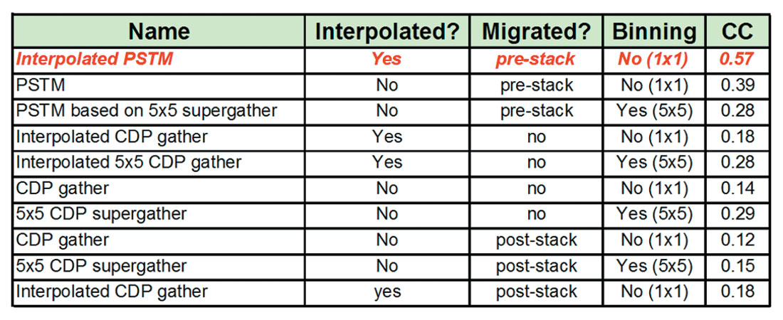
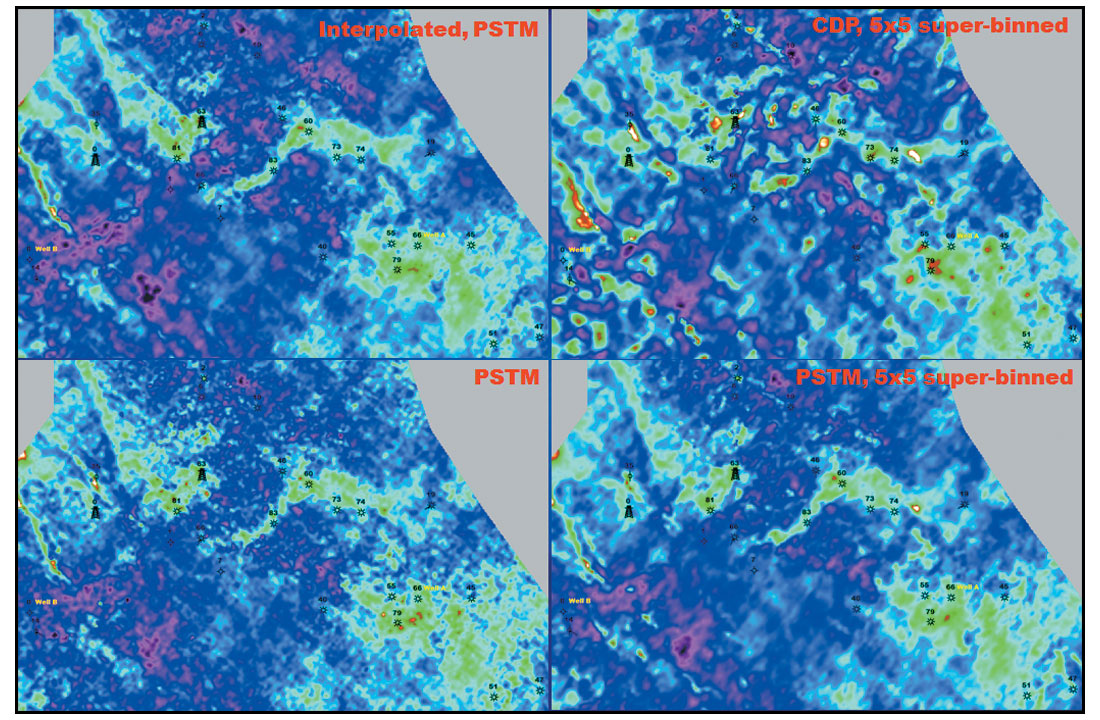
Figure 7 compares a portion of the interpolated PSTM attribute map to the 5x5 superbinned CDP method, the 1x1 PSTM method, and the 5x5 PSTM method. Low ratio values are in green to red. Although the CC values are an objective measure of the veracity of the AVO attribute, they can be hypersensitive to outliers. This is why a comparison of the quality of the map results and even the gathers are of significant additional value. For example, even though the 5x5 CDP method has a similar CC to the 5x5 PSTM method, it is clear from the map comparison that the 5x5 PSTM result is superior. In fact, the map comparsion reveals that the CDP method is grossly inferior to all the PSTM (migrated) results. Wells A and B are also noted, and are discriminated quite well in all maps. The low Rp/Rs ratio trend has a spatially sharp, structurally influenced shape. This spatial sensitivity may be the strongest influence on the dissappointing results of superbinning in this example. Stability enhancement is better achieved prior to migration. In the regression and on the maps, it is clear that the new interpolated PSTM method yielded the best results. The dataset was also used to succesfully predict the results of two new wells denoted with rig symbols on the maps.

The Nisku test case

The 3D that we used for this test had some 14 Nisku penetrations. Of key importance is the fact that 3 of the Nisku penetrations are basinal, and 1 penetration is a tight reef. Each of these wells is given a lithology code as defined in Table 2. We have Pelletier and Gunderson’s Lamé parameter attributes from their original work, and we have the new Lamé attributes extracted from the same 3D with our new interpolation migration technique. We compare the quality of these results in several ways:

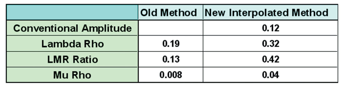
1. The correlation coefficient of (chiefly) the LMR Ratio and (secondarily) the other Lamé parameters to the lithology code that we give to each well on the 3D. This objective, quantifiable measure is illustrated below, in Table 4, and supports improved predictive ability with the new interpolation method. Given the complexity of the mineralogy in the area, and surgical nature of proper use of such Lamé parameters for lithologic prediction, some caution should be taken in evaluating our technique with simple correlation techniques. Nevertheless, this comparison is instructive and supportive of our assertions.
2. Comparison of cross plots of LMR Ratio versus Mu*Rho and Lambda*Rho versus Mu*Rho applied to a map view. These maps are compared and it is shown that the maps resulting from the new method are much cleaner and more geologically reasonable than the old maps (illustrations not shown here ) .
3. The seismic cross sections of Lamé parameters (not illustrated here) demonstrate that the new method has yielded much cleaner, higher signal-to-noise ratio inversions.
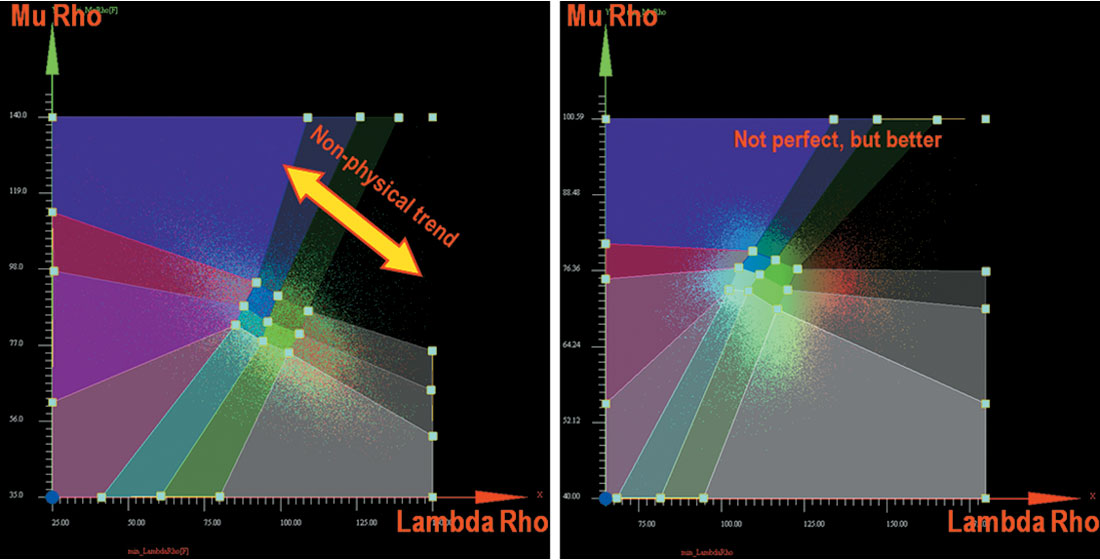
4. The shape and scatter appear in the cross plot domains to also be supportive of our new method. Noise or error in the estimation process contributes to greater scatter of the Mu*Rho axis in particular. These cross plots are compared in Figure 8, below. We know from Figure 4 that we should expect an upper right to lower left set of trends in this particular cross plot space, although mineralogical complexities can cause a widening of the trends in the orthogonal direction. It is clear that the old method has a non-physical trend orthogonal to our expectations, and in excess of what we might expect from the influence of mineralogical variation. The new method yields a more physically meaningful cross plot.

Conclusions

The new interpolation migration method of AVO analysis yielded superior results in our comparative work on the Viking, and the Nisku. In both cases, the signal-to-noise ratio of the new method was illustrated by a variety of methods. The Viking zone had the most well control, and was c o m p a red more rigorously than the Nisku. The well control on our 3D allowed us to validate our method for the Viking objectively, including a quantitative measure of the relationship between Phi-H and an AVO attribute. Of the many variations of the seismic data that we compared, the interpolated PSTM gathers without superbinning were unequivocally the best. Interestingly, the variations that had PSTM were consistently superior to those which were not migrated. Despite our original opinion that imaging would be important, we were nevertheless surprised by how important it was on this data. Interpolation was also shown to be a better method of stabilization than simply superbinning the PSTM gathers. In fact, despite giving the map views a cleaner appearance, the net effect of superbinning did not consistently help our cross correlations–a result that surprised us. Comparisons of gather quality are consistent with the quantitative measures, and support the interpolation PSTM flow that we advocate. Cross plot comparisons of Lamé parameters for the Nisku zone also appeared to physically indicate the superiority of the new method.

AVO attributes are generally of great fundamental importance in seismic interpretation, but their accuracy limits their wider use. This new interpolation method yields measurable improvements to the fidelity of AVO extractions on two zones in related 3D data, and appears to be an important step in enabling wider use of AVO attributes in exploration and development.

It is important to point out that successful interpolation requires the capability of detecting data coherency across spatial dimensions, which heavily depends on successful noise attenuation and static corrections. Therefore, the existence of efficient interpolation tools does not diminish the importance of acquiring data with the best possible sampling. In fact, interpolation could be taken into account during acquisition not to save acquisition costs, but to acquire additional data that can be used by interpolation to infill areas where shots or receivers cannot be deployed. It is better to acquire actual data whenever possible (and economic) due to potential non uniqueness, than to rely too heavily on interpolation.

Future work is focused on using interpolation to precondition the data for azimuthal migrations and analysis (e.g. azimuthal AVO and velocity analysis). This will place greater demands on the interpolation and seismic data acquisition.

Acknowledgements

We thank Scott Cheadle, Kendall Rogers, Xiaowei Luo and John Zhang (CGGVeritas), Cameron Demmans, Brad Molnar (Fairborne) for their work on this project, CGGVeritas Library Canada and Fairborne Energy Ltd for allowing us to show this information.