International Exploration and Expatriate Recruitment and Effectiveness: The Overseas Assignment

Summary

A nonstationary generalization of the convolution integral is presented. Called nonstationary convolution, it forms the scaled superposition of impulse responses, whose form can vary arbitrarily with time or position, 'and has stationary convolution as a limiting form. An alternate formulation is also given, which has the same limiting form but does not have the immediate interpretation of forming the superposition of impulse responses. Called nonstationary combination, this alternate form is closely approximated by the common practice of forming a nonstationary result by interpolation between a set of stationary filtered results. Both filter forms can be re-expressed in a mixed time-frequency domain where nonstationary convolution becomes a generalized forward Fourier integral and combination is a generalized inverse Fourier integral. Additionally, both nonstationary filter forms are re-expressed in the full Fourier domain in a result which generalizes the convolution theorem. A windowing analog is introduced which expresses both filter forms in the case when the nonstationary filter consists of an arbitrary number of piecewise constant stationary filter segments. A set of windows are computed, one for each filter segment, which are unity where the filter segment is applied and zero otherwise. Nonstationary convolution then consists of windowing the input data for each filter segment, applying the corresponding stationary filter to each windowed result, and superimposing. In contrast, nonstationary combination applies each filter specification to create a set of filter panels, windows each panel, and superimposes the results. The possible applications of this methodology are illustrated with examples of wave propagation and deconvolution.

Introductory Concepts

The digital filtering of discretely sampled data is arguably one of the most important processes in geophysical data processing. Examples include temporal or spatial bandpass filtering, deconvolution and wavefield extrapolation (downward continuation). Commonly, filters are of the conventional or stationary variety which means that the filter's form (impulse response) does not change with space or time. Stationary filtering uses the convolution integral to convolve (or filter) one signal with another. Usually one Signal is called the filter and the other is called the input though the symmetry of the convolution integral makes this designation arbitrary. Conceptually, convolution can be described by replacement. This refers to the process of replacing each point on the input signal by a scaled copy of the filter. The scalar is the input sample, the copy of the filter is called it's impulse response, and the output is the superposition of all such scaled filter copies.

The requirement that a filter's form not change with space or time is often too restrictive to model real earth processes. This leads to the desire for nonstationary filters whose properties change, in a controlled fashion, with time or space. Two common uses of nonstationary filters are time-variant deconvolution and space-variant wavefield extrapolation. There are many other possibilities. A common, intuitively-based approach has been to break the data into panels (or segments), apply an ordinary, stationary filter to each panel, and then recombine the panels. Good results are often obtained in this way though the process can be unsatisfactory when the filter must vary rapidly. The lack of a coherent theory of nonstationary filtering, as an extension of stationary filtering, has made the filter panel approach difficult to control in many cases.

Difficulties in dealing with the filter panel approach have lead many scientists to experiment with methods which apply nonstationary filters by first performing a nonstationary transform. A nonstationary transform is one which decomposes a signal on a grid of time and frequency (or alternatively, space and wavenumber). This can be contrasted with the ordinary Fourier transform which decomposes a signal only in a single dimension of frequency. Examples of nonstationary transforms are the wavelet transform and the Gabor transform. Once a nonstationary transform has been done, a nonstationary filter is simply a mask which is applied to the time-frequency spectrum to accentuate or reject selected regions. An inverse nonstationary transform completes the process.

Though very useful, nonstationary transform methods are not the only possibility as is evidenced by the filter panel approach. This suggests that there must be a more comprehensive theory of filtering than the standard stationary theory commonly found in textbooks. Such a theory should describe stationary filters as one end-member of a continuum of possibilities which become progressively more nonstationary. The theory should describe how to specify a filter's properties and how to apply the filter in either the time or the frequency domain. (Here, frequency domain refers to the common domain of the ordinary Fourier transform and not the time-frequency domain of a nonstationary transform.)

At first, it may seem puzzling that we could apply a nonstationary filter in the frequency domain. In a fundamental result called the convolution theorem, a stationary filter can be applied in the frequency domain by multiplying the spectra of the signal and the filter; however, the theorem is usually stated without an extension to nonstationary filters. That nonstationary filters can also be applied in the frequency domain is indicated by another fundamental result from Fourier theory which says that the Fourier transform (or spectrum) is a complete description of a signal. It follows that, if nonstationary filtering can be done at all, it can be done in the frequency domain. A reasonable expectation is that, while stationary filters become a simple multiplication in the frequency domain, nonstationary filters must be a more complicated process.

Over the past several years, our research has resulted in the development of just such a theory of nonstationary filters and we have explored its application in the context of time variant filtering, nonstationary deconvolution, and wavefield extrapolation for depth migration. The theory of nonstationary filters is presented in a mathematical fashion in Margrave (1998). We have also given initial reports of our work on nonstationary deconvolution in Margrave and Schoepp (1997) and on wavefield extrapolation in Margrave and Ferguson (1997). This article contains a conceptual discussion of the basic elements of the theory and illustrates explicitly the correction with filter panels. Though we will present equations, we do so only in summary fashion and invite the reader to consult our technical papers for derivations. Some of the content of this article is very similar to Margrave (1998) but we hope that it is presented in a more accessible manner. Also, the windowing analog, presented in the final section here, is entirely new and offers a very useful intuitive view of nonstationary filtering.

Generalizing Convolution

The key point of departure from stationary to nonstationary filters is an appropriate generalization of the convolution process. There are at least two reasons for the overriding importance of convolution in geophysical data processing, one very practical and one quite theoretical. First, the practical reason is the suppression of random or coherent noise (or, alternatively, the enhancement of signal). Typically signal is bandlimited by the source d1aracteristics while random noise may be broadband. Also coherent noise may contaminate only a portion of the signal band. In both cases, filters may be designed to reject noisy portions of the spectrum while retaining a usable portion of the signal.

The theoretical reason for the importance of convolution lies at the heart of mathematical physics. Physical phenomena are held to be well modeled by a few linear partial differential equations (PDE's). For example, elastic wave propagation is described by the elastic wave equation and this can usually be reduced to a set of scalar wave equations for the elastic potentials. Similarly, the gravitational potential is modeled by Laplace's or Poisson's equations. Also of interest is the diffusion equation for the description of heat flow and the scalar wave equation for acoustic waves. A powerful solution technique for any linear PDE, known as Green's function theory, turns out to be a convolution or filtering process. Essentially, the theory states that if the solution to the PDE for an impulsive source can be found, then the solution for a more general, distributed, source is obtained by filtering the impulsive solution. The impulsive solution is called a Green's function (or impulse response) and the distributed source becomes the filter.

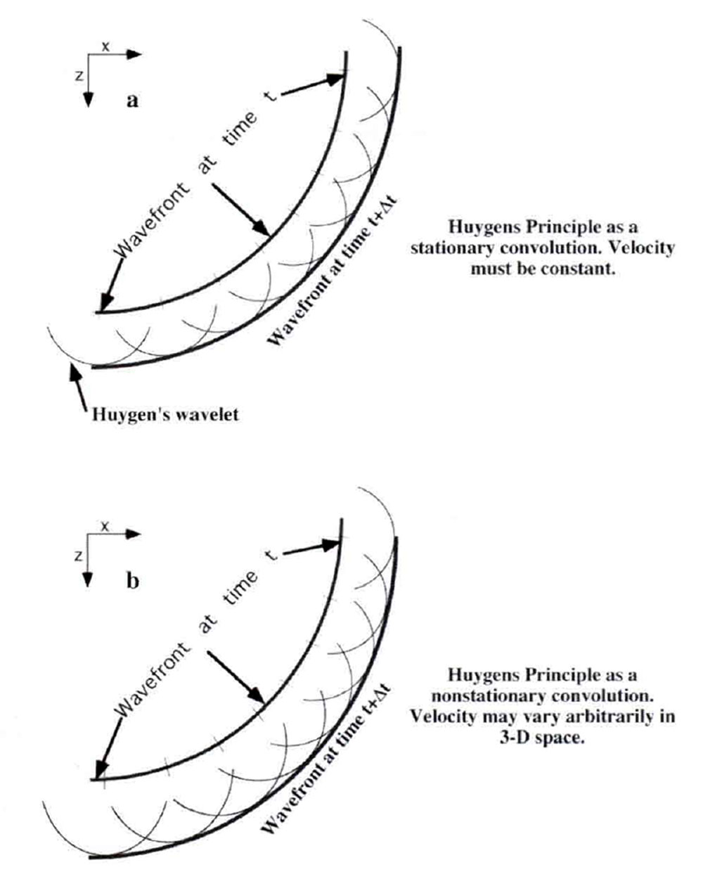
An intuitive example of this Green's function theory is the propagation of waves through the application of Huygen's principle (Figure 1a). A wavefront can be stepped forward in time (i.e. extrapolated) by considering each point on the wavefront to be an impulsive source and a new wavefront is synthesized from the superposition of all such sources. Thus the wave is stepped forward by filtering the input wavefield with an appropriate Green's function, which may be called a Huygen's wavelet. The extrapolated wave is constructed as the linear superposition of all possible Huygen's wavelets, each one representing an expanding spherical wavefront about a point on the input wavefield. Clearly, the radius of the Huygen's wavelet must depend on the local wave propagation velocity and can only be constant if velocity is constant. In the constant velocity case, this process is a multi-dimensional convolution by replacement. In the variable velocity case, it is still a linear superposition of Huygen's wavelets but each varies its radius according to the local wavespeed (Figure 1b).

This physical argument serves to define the desired properties for nonstationary convolution. It must be an integral form which tends smoothly to the stationary convolution integral as the filter becomes stationary. Also, it must have the physical interpretation of forming a scaled superposition of impulse responses whose form varies with time or space.

Time Domain Forms of Nonstationary Filtering

In order to understand what a nonstationary filter is, we must first clearly understand what a stationary filter is. The convolution of a stationary filter a(t) with an input function h(t) to yield g(t) is given by

Note that the filter is dependent only on "lag time" t-τ:. If we consider the case when h(τ) = cδ(τ-τo) (where c is a constant and δ is the Dirac delta function), then g(t)=ca(t-τo). This deceptively simple result has far reaching effects and is the basis for most numerical convolution algorithms. In words, if the input to a convolution is an impulse of magnitude c at time τo, then the output is the filter function scaled by c and shifted to τo. Thus the filter function is scaled and translated (shifted to τo ) but is otherwise unchanged. For this reason, a(t) is often called the "impulse response" of the filter since it is the result when h(τ) = δ(τ). This result generalizes to arbitrary input functions by considering them to be the superposition of a set of impulses and captures the essence of a stationary filter. Simply put, a stationary filter keeps the filter's form invariant and replaces each point on the input function with a scaled copy of the filter. The output is the superposition (summation) of all such scaled and shifted filter functions.

Returning to the Huygen's principle discussion from the previous section, the Green's function (or filter or Huygen's wavelet) represents an expanding wavefront of radius vΔt where v is the velocity and Δt is the extrapolation time step. If v is constant, then the spherical wavefront will have a constant radius no matter where it is placed on the input wavefront. Thus, in this case, stationary convolution is an appropriate mathematical tool to form the required scaled superposition of Huygen's wavelets. However; when velocity is allowed to vary from point to point, as it obviously does in the earth, then the radius of the wavefront must vary and stationary convolution cannot provide the needed flexibility. A mathematical process which can form a scaled superposition of Huygen's wavelets (or any other filter) while allowing the wavelet radius to depend on the local velocity at the point of replacement is called a nonstationary convolution (Figure 1b).

A nonstationary convolution integral is needed which symbolizes the nonstationary filtering processes just discussed. It must allow the filter to depend on both input and output time and not merely their difference. Additionally, it must retain the meaning of replacing each input point with an impulse response and should approach equation (1) in the "stationary limit". To deduce a more general form, we can expand the role of the impulse response discussed previously. Now, when an impulse h(τ) = cδ(τ-τo) arrives, we would like to have a response something like g(t) = ca(t-τo, τo).

That is, the response changes according to both the lag time and the impulse time. This suggests that equation (1) be generalized to

Equation (2) is called nonstationary convolution because it meets all of the criteria which were required: it is linear, it allows the filter to depend on both input time and lag time, it has equation (1) as its stationary limit, and it forms the scaled linear superposition of impulse responses. Thus we have generalized the concept of the impulse response function in equation (1) to a two dimensional function a(u,v), where u and v are generalized time variables. The interpretation of a(u,v) is that it prescribes the response of the linear system, without the causal delay, to an impulse arriving at time v. This is convenient because it allows the impulse responses at different times to be directly compared (Figure 2) and we incorporate the causal delay into the integration form of equation (2). The stationary limit is found by letting the v dependence become constant.

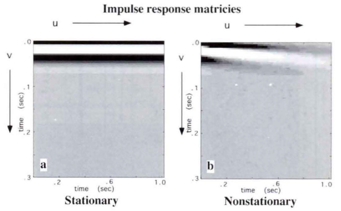
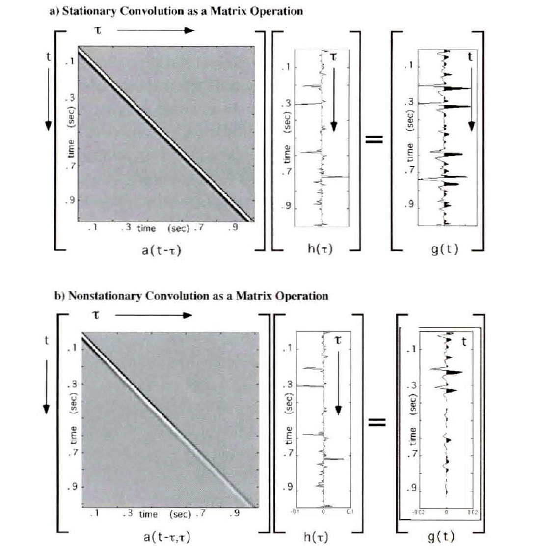
Figure 3 illustrates the discrete approximations to equations (1) and (2) being computed as matrix-vector multiplications. In Figure 3a, the stationary impulse response matrix of Figure 2a has had each column delayed to place the filter start-time on the main diagonal, creating a Toeplitz matrix. The resulting matrix multiplies the input signal to complete the convolution of equation (1). In Figure 3b, the nonstationary convolution is also a matrix operation. The nonstationary convolution matrix is formed by delaying each column of the impulse response matrix of Figure 2b but no longer has the Toeplitz symmetry.

There is another linear form, similar to equation (2), which is of considerable interest because it appears in many data processing algorithms. Called nonstationary combination, it is given by

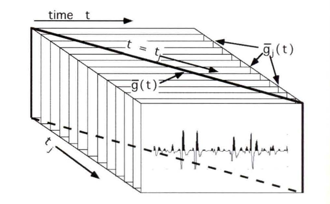
Nonstationary combination differs from convolution in that it maps the v dependence of a(u,v) into output time rather than input time. Though this difference vanishes in the stationary limit, it can be dramatic for highly nonstationary filters. The response of equation (3) to h(τ) = cδ(τ-τ:o) is g(t)= ca(t-τo, t) rather than g(t) = ca(t-τo, τo) for equation (2). Given the interpretation of a(u,v) mentioned above, equation (3) cannot be regarded as forming the superposition of impulse responses since the v dependence is not mapped to the arrival time of the impulse. As will be demonstrated below, nonstationary combination is closely related to the filter panel approach. In fact, nonstationary combination is exactly formed by slicing through an exhaustive (or complete) set of filter panels as shown in Figure 4.

Though applying the same filter form as a combination or a convolution can give very different results, it is also true that a convolution filter form can always be constructed which will give identical results to a combination filter and vice-versa. That is, if h(τ) is filtered with a(u,v) using equation (3) to get g(t) it is always possible to find a filter, a(u,v), which can be applied with equation (2) to yield the identical result g(t). Therefore, though combination does not form the linear superposition of impulse responses of the filter a(u,v) in equation (3), it does form the linear superposition of the impulse responses of a related quantity a(u,v).

Mixed-Domain Forms of Nonstationary Filtering

The two forms of nonstationary filtering introduced above are very closely related. Both are linear and both have stationary convolution as a limiting form. However; when a nonstationary impulse response function, a(u,v), is applied with equation (2) or, alternatively, with equation (3) the results can differ strongly. More understanding follows from reformulating these expressions in the Fourier domain and, as an intermediate step, we will now present mixed-domain forms for both operations. The name is meant to imply that the domain of the signal changes during the application of the filter, either from time to frequency or the reverse. First we define conventional forward and inverse Fourier transforms

Note that the spectra of g and hare G and H and that, corresponding to the input time, is the input frequency η while the output time, t, has frequency f.

The mixed-domain form of nonstationary convolution follows by using equation 5a to take the forward Fourier transform of equation (2). After some math, the resulting expression is

where

In equation (7), u and v are the generalized times mentioned before and p is a frequency corresponding to u. At first, it may seem odd to write equation (7) in terms of such generalized quantities instead of the f and τ required in equation (6) but this will allow the same expression to be used later for nonstationary combination much as a(u,v) was used in both equations (2) and (3).

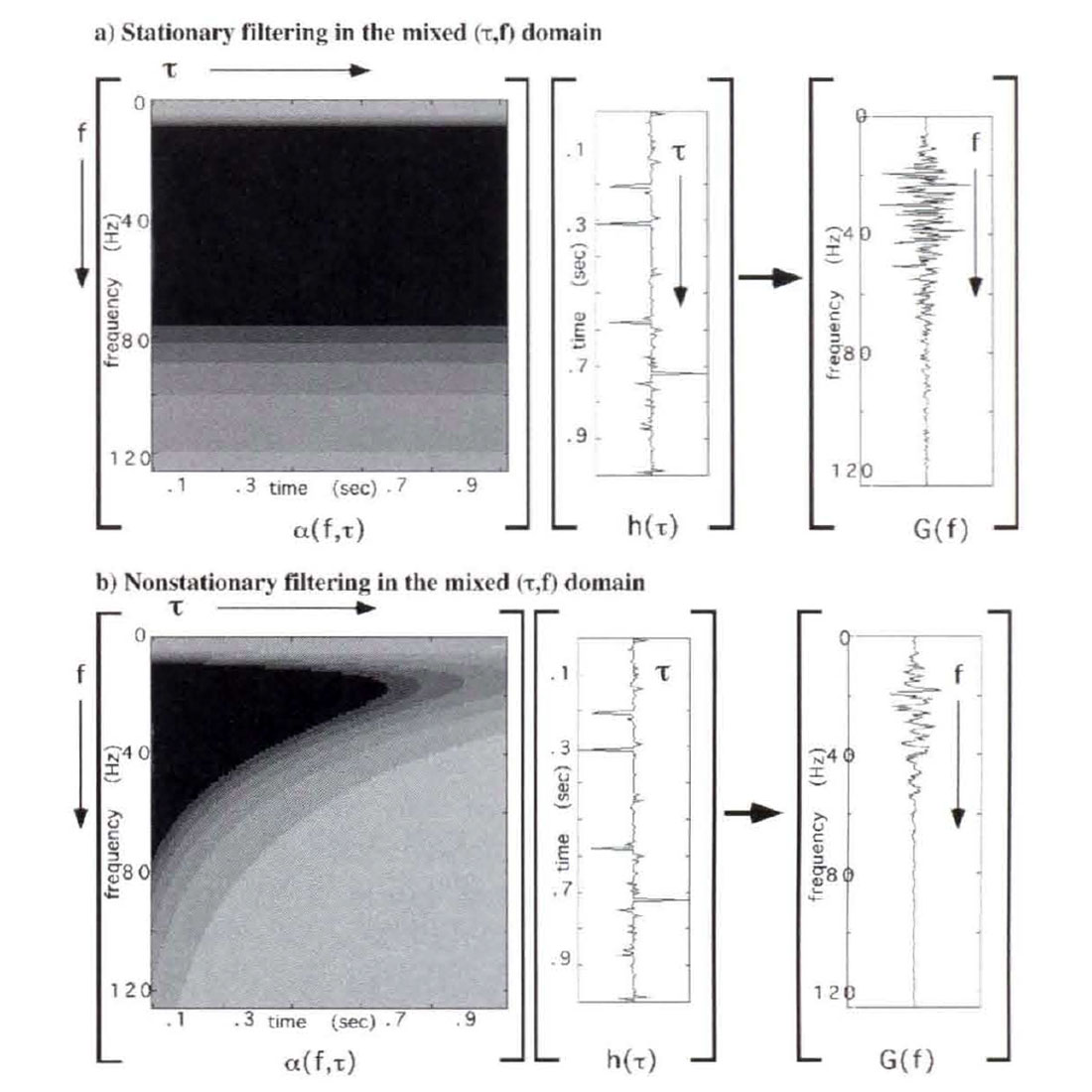
Equation (6) is the mixed form for nonstationary convolution and it uses α(p,v) with P mapped to f and v to τ. First note that if the v dependence of α(p,v) becomes constant (i.e. the stationary limit) then α(f) can be taken outside the integral and we have the ordinary forward Fourier transform of he,) times a filter function α(f). That is, we get the expected stationary result that the filter is applied by multiplying the spectra. More generally, α(p,v) depends strongly on both p and v and, as equation (6) shows, it is applied simultaneously with the forward Fourier transform of the input function h(τ). The final output signal g(t) is obtained as the ordinary inverse Fourier transform of G(f) as in equation (5b).

As defined by equation (7), α(p,v) is the ordinary Fourier transform over the first time coordinate of the impulse response function and is called the nonstationary transfer function. That is, α(p,v) gives the Fourier spectrum of the impulse response for each impulse arrival time v. There are few restrictions on the nature of α(p,v) so that nearly arbitrarily complex spectral functions can be applied and they may vary arbitrarily with time. (The only restrictions required are those sufficient to make the integrals converge and to allow their interchange.) Since equation (7) is an ordinary Fourier transform, it is easily inverted to give a(u,v) in terms of α(p,v).

Figure 5 illustrates the application of stationary and nonstationary filters through the discrete equivalent matrix operations for equation (6)..

The mixed-domain form of nonstationary combination is derived by substituting for h(τ) in equation (3) its expression as an inverse Fourier transform of H(η) as given by equation (4b). Again, we omit the derivation and quote the result:

This result contrasts strongly with equation (6). In both cases the same nonstationary transfer function is involved; however in equation (6) it is applied simultaneously with the forward Fourier transform while in equation (8) it is with the inverse Fourier transform. Furthermore, note that the integration in equation (6) involves the v dependence of α(p,v) while equation (8) integrates over the p dependence.

Fourier Domain Expressions

In this section, we will move these nonstationary filter forms, convolution and combination, entirely into the Fourier domain. (The derivations are given completely in Margrave, 1998.) The result is that nonstationary convolution becomes

where

Equation (10) defines the frequency connection function, A(p,q), which determines the connection or mapping between input and output frequency. A(p,q) may be computed from a(p,v) by an ordinary Fourier transform over v or, equivalently from a(u,v) by a 2-D Fourier transform over u and v.

The comparable expression for nonstationary combination in the Fourier domain is

The subtle difference between equations (9) and (11) is very intriguing. Both can be seen to be nonstationary filter forms which are mathematically similar to the time domain expressions of equations (2) and (3). In fact, nonstationary convolution has a combination form in the Fourier domain and vice-versa for nonstationary combination.

Figure 6 shows the discrete computations of both a stationary and a nonstationary filter by equation (9) as matrix operations. The filter being applied is the same as in Figures 3 and 5. In the stationary limit, A(p,q) becomes A(p)δ(q) (Margrave, 1998) and the integral in equation (9) collapses to a scalar multiplication. For a discrete application, this becomes a diagonal matrix multiplication as shown in Figure 6a. If the diagonal were displayed in profile, the spectrum of the stationary filter would be seen. In the nonstationary case, the filter matrix can have significant power everywhere, though it will be diagonally dominant for a large class of quasi-stationary filters.

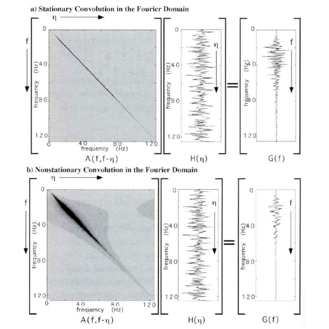
Comparing the matrices in Figures 3 and 6, we can appreciate that as the stationary limit is attained, the convolution matrix becomes Toeplitz, and the spectral matrix becomes diagonal. In a general nonstationary setting, both matrices are non-Toeplitz and are potentially fully populated.

Equation (10), like equation (7) moves the nonstationary filter specification between domains using ordinary Fourier transforms. As such, these equations can easily be inverted and provide general prescriptions for moving a filter between domains. It is usually preferable to design the filter in the mixed-domain and then move it to either the Fourier or time domains for application. The choice of domain for filter application can be made on considerations of computational efficiency. The domain in which the filter application matrix is more nearly diagonal will usually be preferred.

The Windowing Analog

The mixed-domain filter forms, equations (6) and (8), are conceptually rich and offer great flexibility in the design of filtering algorithms. Considerable insight can be gained into the distinction between the convolution and combination forms by analyzing the simple case

Here α(p,v) is composed of two stationary filters, discontinuously juxtaposed at v = 0. First, compute nonstationary convolution from equation (6)

Now define two window functions

Using these window functions, equation (13) can be rewritten as

in which the integrals are now ordinary forward Fourier transforms. If we let FT denote a forward Fourier transform and IFT an inverse Fourier transform, then the final filtered result in the time domain is

This result has an obvious generalization to the case where α(p,v) consists of any number of piecewise constant segments. In this case, it shows that nonstationary convolution can be formed from a set of stationary operations by windowing the input dataset to select that portion corresponding to each stationary filter segment, filtering the windowed segment, and superimposing the results. (Since the inverse Fourier transform is linear, the summation and the IFT can be interchanged in equation (16).)

Now consider the computation of nonstationary combination with equation (8) for the filter form of equation (12). In this case, equation (8) becomes

Using the window functions of equation (14), equation (17) can be written as a single specification

and this result can be written in a form similar to equation (16) as

As before, this result can easily be extended to an arbitrary number of piecewise constant filter segments.

Equations (16) and (19) offer an intuitive understanding of the essential difference between nonstationary convolution and combination. Suppose that the nonstationary filter specification can be written as piecewise constant (in time), that is, as a countable number of stationary filter spectra defined over time zones. Next, define a set of window functions, one for each stationary filter such that the window is unity over the specification zone of the filter and zero elsewhere. A nonstationary convolution is computed by windowing the input dataset, filtering each windowed result, and superimposing them. In contrast, a nonstationary combination proceeds by filtering the input dataset (without windowing) with each filter specification, windowing the filtered results, and superimposing. Imagine an input dataset that contains a single live sample (an impulse) which falls in the middle of the jth filter specification zone. Suppose further that the impulse responses of each stationary filter are very long in time such that they easily span the specification zones of many other filters. The nonstationary convolution will simply be the impulse response of the jth stationary filter since only the jth window applied to the input data will contain nonzero energy. However; nonstationary combination gives a much different answer. Since the stationary filters in equation (18) are applied before windowing, each will produce its own impulse response of the single live input sample. The application of windows after-the-fact will result in a composite "impulse response" which changes discontinuously at each filter specification boundary. Nonstationary convolution offers a powerful method of solution to physics problems which can be superior to nonstationary combination because the former creates a scaled superposition of impulse responses while the latter does not.

A general property of a combination filter, suggested by the previous paragraph, is that any discontinuities in a(p,v) in the time direction (v) will result in discontinuities in the filtered output. Thus it is possible to produce a completely abrupt change in the time domain output. Nonstationary convolution cannot show this behavior since the continuous superposition of impulse responses will smooth over any filter discontinuities. This observation explains much of the objectionable behavior of the filter panel approach when the filter must change rapidly.

As an example, the method of wavefield extrapolation by phase shift (Gazdag, 1978) can be extended to nonstationary phase shift (NSPS) (Margrave and Ferguson, 1997) by simply replacing v by v(x) (v is velocity) in the constant velocity expression and formulating it as a convolutional expression. The same nonstationary wavefield extrapolator, when applied as a nonstationary combination leads to the method of PSPI (Gazdag and Squazerro, 1984).

Figure 7 illustrates the development of wavefield extrapolation through the windowing method of nonstationary combination. In Figure 7a, an input dataset consisting of three isolated impulses is ready for downward continuation by wavefield extrapolation. The wave propagation velocity is assumed to consist of three regions of different constant velocities centered on each impulse. It is a standard result from wavefield theory, that, for constant velocity, this can be done by a 2-D filter whose shape (or impulse response) is an upside-down diffraction hyperbola. In Figure 7b, the input has been filtered with an operator whose shape is determined by the velocity V_low, and in Figure 7c a window has been applied to select only the result where V_low was the correct velocity. This process is then repeated in Figures 7d and 7e for velocity V_med, and Figures 7f and 7g for velocity V_high. The change in the shape of the diffraction curve is directly controlled by the local velocity. The final result in Figure 7h is the summation of the wavefields in Figures 7c, 7e, and 7g. This completes the implementation of equation (19). Wavefield discontinuities can be seen in Figure 7h at the location of the velocity step boundaries.

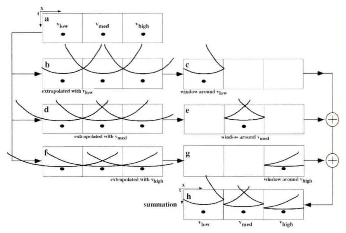
Figure 8 is a similar development of wavefield extrapolation by nonstationary convolution resulting in the NSPS algorithm mentioned previously. (The input wavefield and the propagation velocities are the same as for Figure 7; however, the process applies equation (16) rather than equation (19).) In Figure 8b, the input wavefield is windowed to isolate the portion corresponding to velocity vlow, and in Figure 8c the result is filtered with the wavefield extrapolation filter for vlow. This process is repeated for the remaining velocities and the final result, Figure 8h, is the summation of the windowed and filtered results for each constant velocity. A superposition of constant velocity impulse responses has been achieved and there are no wavefront discontinuities.

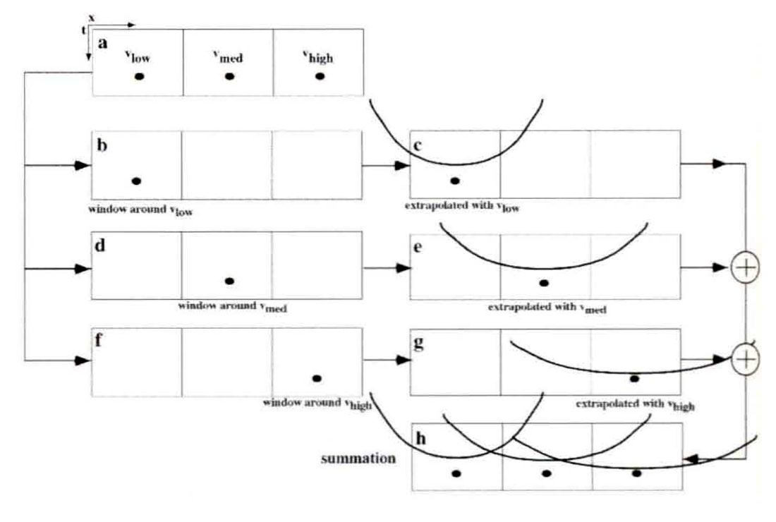
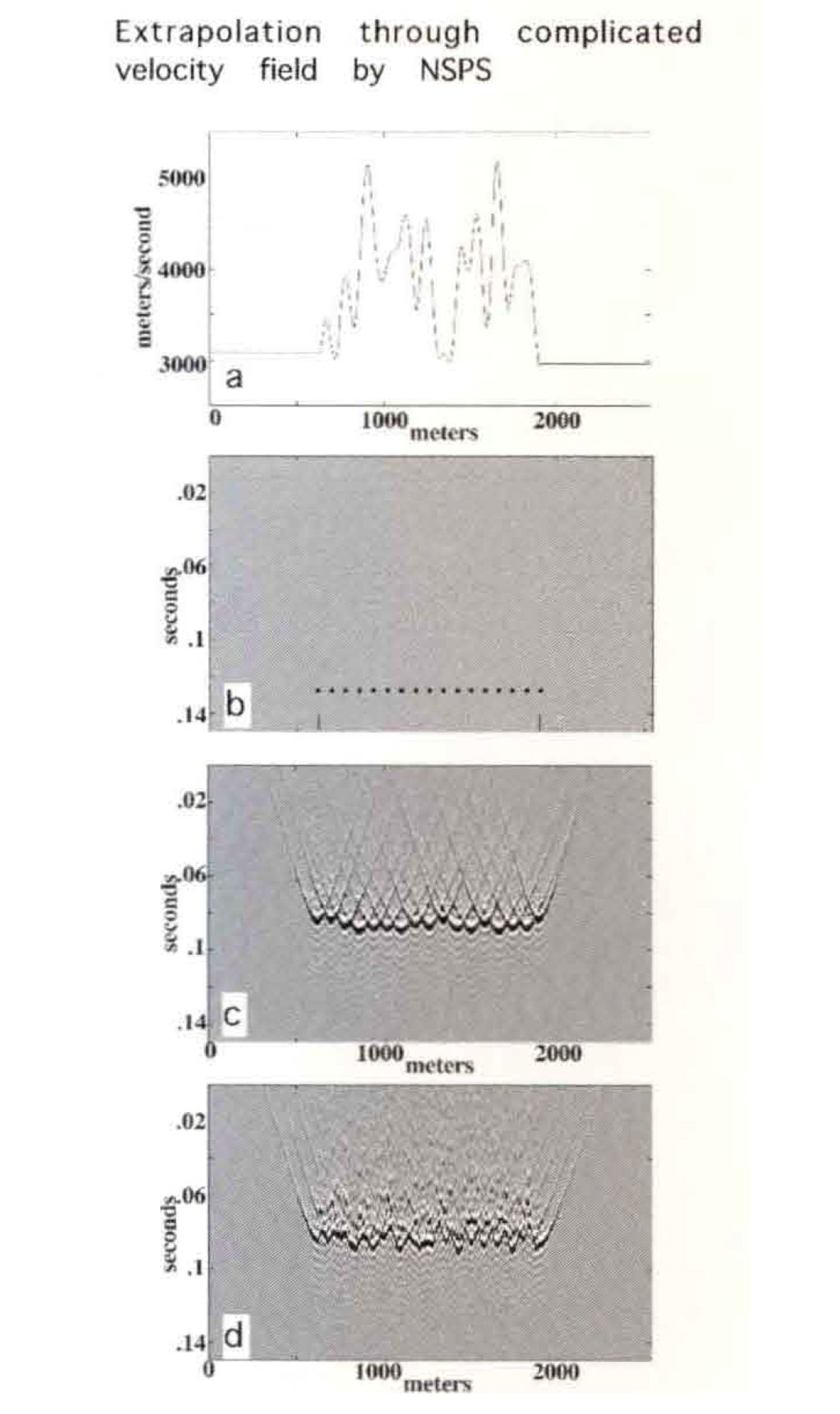
Figure 9 shows an actual numerical computation using NSPS and PSPI for a velocity field which varies rapidly with lateral position but is constant vertically (Figure 9a). Though the windowing analog provides a complete conceptual understanding, this computation was actually performed in the Fourier domain using equations (9) and (11). Figure 9b is a row of impulses which will be extrapolated through a single 50m vertical step with both methods. The NSPS result (Figure 9c) can be seen to be a superposition of hyperbolic impulse responses while the PSPI result (Figure 9d) is relatively chaotic.

We remark that neither NSPS or PSPI have been developed directly from a variable velocity wave equation. Rather, they are two alternate extensions of the exact constant velocity phase shift method into the variable velocity case. Both methods are intuitive approximations and neither is capable of responding to local velocity gradients. However, we feel that SPS offers some distinct advantages over PSPI, most notably in algorithmic stability. We will be investigating and improving these methods in the future.

Elsewhere, Margrave and Schoepp (1997) and Schoepp and Margrave (1997) have demonstrated that robust and useful deconvolution routines can be built based on these ideas (Figure 10). This approach merges the ideas of stationary frequency domain deconvolution and inverse Q filtering. The result is an algorithm which can deconvolve the source waveform, compensate for both the amplitude and phase effects of absorption, and address a wider class of multiples than conventional deconvolution. Moreover, it does not require the precise knowledge of Q that inverse Q filters typically need. Such a nonstationary deconvolution approach promises higher resolution seismic images with a stationary embedded wavelet and more meaningful reflection amplitudes.

Conclusions

The concept of convolution is important to seismic data processing as a filter application technique; but more importantly, plays a central role in physical theory The solutions to the partial differential equations of physics can be written as convolutions of an impulse response with a source distribution. When the coefficients of the equation, which are determined by the physical parameters of the medium, are constant, the convolution is stationary and the solution is often exact When the coefficients vary with space or time, the convolution is nonstationary and the solution is generally approximate.

Nonstationary filter theory provides a complete methodology for description and application of nonstationary filters. The convolution form of nonstationary filters results in the scaled linear superposition of the nonstationary impulse responses. An alternate filter form, nonstationary combination, still forms a linear superposition but does not preserve the filter's impulse responses. Both nonstationary filter prescriptions reduce to stationary convolution in the stationary limit The theory provides arbitrary control of the time and frequency characteristics of the nonstationary filter and applies the filter without having to decompose the signal with a nonstationary transform. Only stationary Fourier transforms enter into the theory.

Nonstationary convolution becomes a generalized forward Fourier integral when moved into the mixed-domain of time-frequency. This expression applies the nonstationary filter simultaneously with the Fourier transform of the signal from the time domain to the frequency domain. Nonstationary combination is a generalized inverse Fourier integral which moves the signal from the frequency to the time domain while applying the filter.

Nonstationary filters can also be expressed in the full Fourier domain. If the time domain discrete filter matrix is Toeplitz (stationary) the Fourier domain filter matrix is diagonal and vice-versa. The preferred of domain of application of nonstationary filters is that in which the filter matrix is most nearly diagonal.

For a nonstationary filter whose temporal variation is piecewise constant, the mixed-domain forms can be manipulated to produce an intuitive windowing technique of filter application. Given a set of windows, one per filter segment with its passband centered on the filter specification zone, nonstationary convolution windows the data, filters each windowed subset, and superimposes the results. Nonstationary combination, filters the input data with each filter segment, then windows and superimposes. Applied to wavefield extrapolation, nonstationary convolution (NSPS) produces a dramatically superior result to a combination approach (PSPI).

Nonstationary filter theory holds great promise for many geophysical problems.

Acknowledgements

We thank the sponsors of The CREWES Project for their continued generous support