Influence of Acquisition Geometry on Event Cloud Asymmetry and on b-Value Analysis

The most common setup to monitor microseismic events during hydraulic fracturing experiments includes a single observation well. This type of setup can lead to biases in event detection, location and magnitude computation. We statistically analyse simulated catalogues of events that represent common hydraulic fracturing experiments and especially focus on the symmetry/asymmetry of the event clouds. Results show that the radial orientation of the event clouds with respect to the observation well is the key factor in event cloud asymmetry. The detection threshold due to the distance from the observation well can significantly increase this asymmetry and has a strong influence on the observed magnitude distribution. Using a minimum common magnitude threshold corrects for asymmetry if caused by detection deficiency. The distance-magnitude detection threshold negatively impacts other derived quantities such as b-values.

b-values (coefficients representing the ratio between small and large magnitude events) in excess of 1.5 are likely to be underestimated due to elimination of the smaller magnitude events. Application of a common minimum threshold at all distances can correct for systematic biases in b-values but at the expense of increased estimation variances because of the reduced number of events. The developed simulation strategy can be used to assess potential biases in various statistical parameters due to existing or planned acquisition geometry.

Introduction

Monitoring of microseismic events is widely used to evaluate the success of hydraulic fracturing in oil, gas and geothermal reservoirs and to follow almost in real-time the development of fracture networks (van der Baan et al., 2013). The spatial distribution of events is thought to reflect the fluid induced fractured zone in the reservoir (Cipolla et al., 2011). The distribution of magnitudes is used to make inferences on the in-situ changes in the stress field (Grob and van der Baan, 2011) or to distinguish between fluid injection or fault reactivation related events (Maxwell, 2012) through the value of the fractal dimension b that quantifies the ratio between large and small events. But care should be taken when interpreting the shape and attributes from microseismic events (Cipolla et al., 2011; Zimmer, 2011).

Indeed not all microseismic events are recorded because of energy loss during wave propagation, and often only one observation well is used to monitor the microseismicity, which leads to inaccurate positioning and detection failure for events happening far from that well. Magnitude-detection thresholds could result in systematic biases in b-values. Maxwell (2012) suggests focusing on quality over quantity by normalizing the event pattern using a magnitude cutoff to interpret fracturing. The question is how much information is actually lost with this strategy and how to quantify that loss.

Modeling is a convenient way to quantify information loss. In simulations all events are known and a detection threshold can be specified to mimic the loss in recorded microseismic events due to the distance from the observation well. Quantification can be achieved by computation of systematic biases and uncertainties in relevant parameters. The question of quality over quantity can then be tested by thresholding the event magnitudes with distance and assessing the resulting change in statistical parameters. This can be done for various acquisition setups.

Simulation strategy

Catalogs of events are created to study the influence of acquisition geometry on event clouds. In order to be as close as possible to reality, the event magnitude distribution in the simulated catalogs follow the power-law defined by Gutenberg and Richter (1944) as:

N is the number of events with a magnitude m superior to a certain magnitude M. The value b is the coefficient of the power law and represents the slope of the curve in a semilog plot of N versus M. The parameter a defines the background seismicity. To simulate a catalogue of events obeying equation 1, we define the coefficient b, the total number of events N_tot and the minimum and maximum desired magnitudes M_min and M_max. Scalar a is then given by:

The number of events N_i for each bin ΔM between M_min and M_max is given by:

Random magnitudes are assigned for every magnitude bin for the number of events N_i determined by equation 3. The maximum observed magnitude may be less than the maximum defined magnitude M_max as a minimum of one event has to occur in each bin. A high b value leads to a smaller observed magnitude range. Minor variations between chosen and simulated b-values may occur because Ni has to be an integer but the theoretical N_i could be a float number which has to be rounded.

For simplicity we assume that the microseismic cloud occurs within a horizontal plane. Extensions to 3D clouds are straightforward but do not yield significantly different insights. The two dimensional, spatial distribution of events in our simulations is characterized by an ellipsoid with axes A and B (defined in order of length). A unit circle area is uniformly filled with random points. The circle is then stretched out linearly to form an ellipse with semi-length axes A and B. The spatial distribution of points within the ellipse is thus still uniform. Each point in the ellipse is then attributed a magnitude randomly from the distribution defined above.

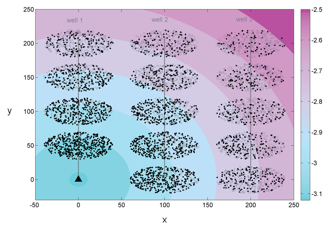
A typical simulation to represent hydraulic fracturing has the following features: one observation well and one cloud of simulated events per stage, parallel to one another and perpendicular to a virtual horizontal well. In our simulations we consider three different horizontal wells: one at the same level as the observation well along the vertical axis (well 1), one 100 units further (well 2) and one 200 units further from observation well (well 3). Figure 1 illustrates the configuration of the simulations. The stage numbers are counted from bottom to top, stage 1 being the closest to the observation well. Well 1 has only four stages as the first one would have been just under the observation well, so for better visualisation this stage was not considered. The other wells have a total of five stages, one of them aligned with the observation well along the horizontal axis.

Next we consider a magnitude-distance threshold given by the following equation:

where slope is the parameter describing the detection limit, and d is the distance between events and geophones. This threshold is shown as the oblique black line in Figure 2, and the parameters slope and Md0 shown in the figure equal 0.002 and -3.15, respectively. It is also illustrated as the colored contours in Figure 1. This detection threshold is then applied to simulate missing events due to distance to the observation well as seen in the magnitude-distance plots for real microseismic events. All events below that line are no longer considered in the analysis. They are shown as gray open circles in Figure 1.

In some cases a minimum common magnitude threshold (horizontal dashed line in Figure 2) is applied to take into account only the high magnitude events as in Maxwell (2012). This threshold corresponds to the lowest magnitude found at the furthest distance above the detection threshold. The purpose of that simple magnitude cutoff is to ensure analyses of events are performed over a homogeneous set of data with similar conditions, which should allow for a more meaningful interpretation (Cipolla et al., 2011; Maxwell, 2012).

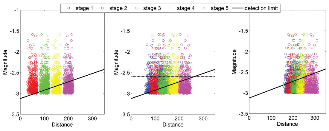
Two examples are shown in the result section, example 1 with a slope parameter of 0.002 and example 2 with a slope of 0.005. The 0.002 value is similar to a slope value found for real microseismic data (see case study section) and the increase in the slope to 0.005 is chosen to illustrate the influence of detection limit on the shape of event clouds for a highly attenuating medium or equivalently a greater distance between the treatment and observation wells. The minimum common magnitudes are -2.6 and -2 in each example respectively.

Results

Event cloud asymmetry assessment

For better visualization the examples shown in the following figures contain only 500 events, and the theoretical b-value chosen for each cloud is 1.8. Figure 1 shows the three different simulation scenarios with colored contours showing the magnitude corresponding to the detection threshold as shown in Figure 2. Figure 1 clearly points out that the radial orientation of an event cloud with respect to the observation well will determine the influence of the detection threshold. Indeed the clusters whose major axis is most aligned to a radial direction from the observation well will be more affected by a detection threshold as they spread over a wider range of magnitude thresholds, thus increasing their asymmetry.

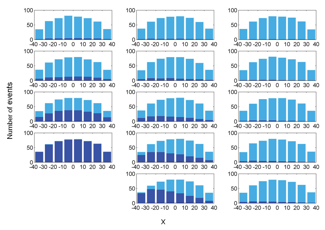
To assess the asymmetry of the clouds after the detection and magnitude thresholds are applied, histograms showing event distributions projected onto the major axis of each event cloud are computed for each stage and each well. The results averaged over 50 iterations are displayed in Figure 3 for example 1. The histograms start out symmetric with slightly higher densities in the center than at the edges due to the elliptic cloud shape if no magnitude thresholding is applied. Clearly event counts decrease with increasing distance from the observation well. Stages with major axis oriented predominantly radially away from the observation well have the strongest asymmetric distributions (e.g. stage 1 of well 2). Stages 5 for every well have a rather homogeneous distribution of events. All stages for well 1 also show a more symmetric event distribution as this well is oriented radially to the observation well such that magnitude thresholding occurs symmetrically along the major axis. Stage 2 of well 1 is least affected by the detection threshold and still contains 500 events, whereas stage 5 of well 3 is most affected due to its distance from the observation well. The number of events is reduced by a factor two between the first and the last stages with the parameters chosen for example 1.

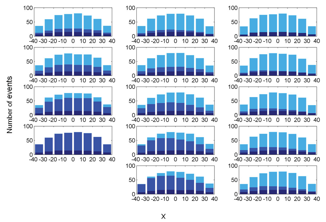
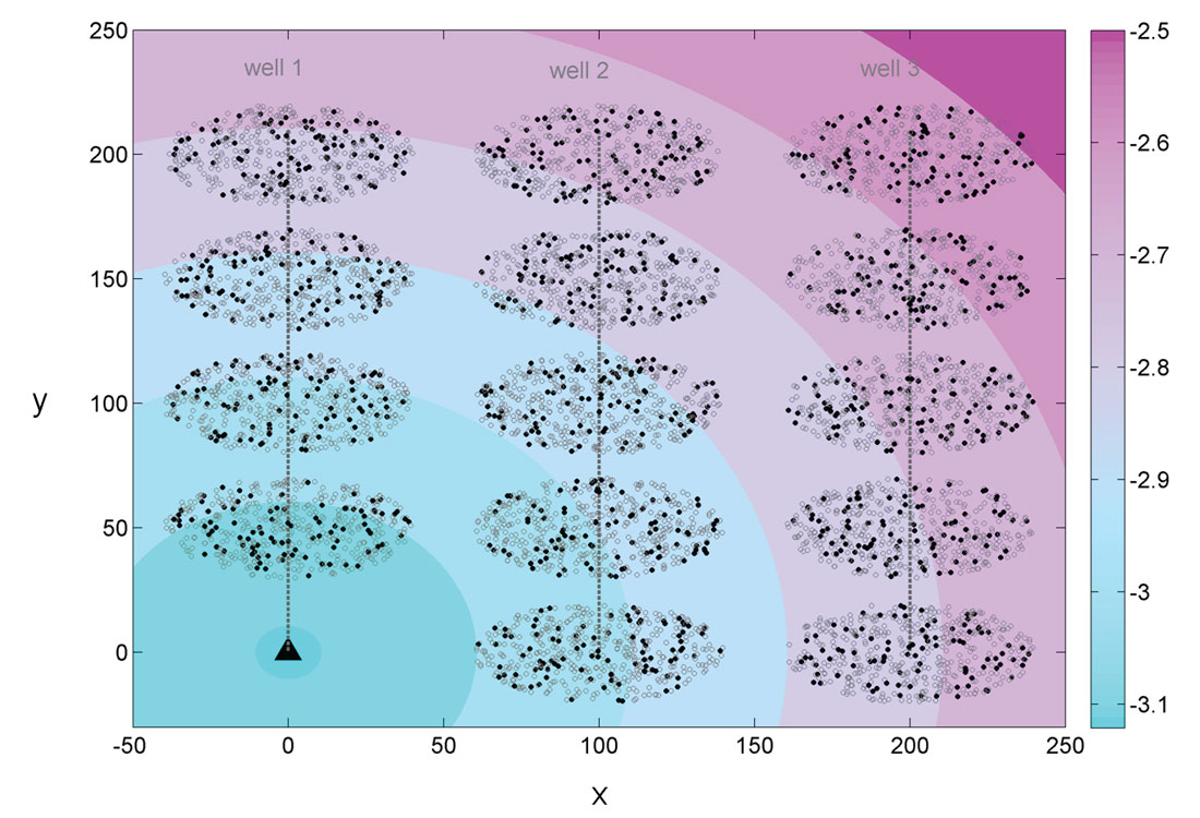
Figure 4 displays in a similar way the removal of events (open circles) after a minimum common magnitude threshold is applied to all observed events as suggested by Cipolla et al. (2011) to remove potential biases due to the distance-magnitude threshold. As all clouds of events obey the same Gutenberg-Richter relation, the same number of events is left in all clusters after the magnitude threshold (94 events are still in the clouds in this particular example). The distributions of events along the cloud major axis for all stages are more symmetric than after the detection threshold is applied (Figure 3). This is due to the magnitudes being randomly attributed to spatial points and produces a more similar distribution to the true one.

Next we consider the case of more severe magnitude thresholding with distance (or equivalently wells and clouds spaced out over a larger area). If the slope of the detection threshold line in Figure 2 is doubled (here set at 0.005 for example 2), the removal of events is even more dramatic. There are only very few events left in the far-out stages in this scenario. The corresponding distributions of events along the cloud major axis display an increasing asymmetry (Figure 5) with no remaining events in the right part of the cloud (between 10 to 40 units) for stages 4 and 5 of well 3. The histograms for well 1 are still characterized by a more symmetric distribution as expected given the well orientation. The reduction in observed events for wells 1 and 2 is two orders larger than for the stage 1 of well 1 and for the previously considered scenario with a more gentle distance detection threshold.

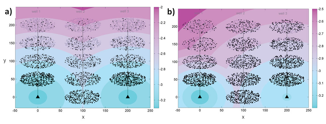
One solution to increase the number of recorded events is to use a second monitoring well. Figure 6 displays contour plots with corresponding clouds of events when two observation wells are in place. Two scenarios are considered here, one where the detection slope is the same from both observation wells (Figure 6(a)) and one where detection slopes are different (which could be due to anisotropy, different laterally distributed rock properties or simply mimicking an increased distance to the observation well; Figure 6(b)). The use of two observation wells clearly increases the amount of events recorded and improves the symmetry of event clouds which would lead to better interpretation of event locations, even in the case of two different detection slopes. However these events are recorded by at least one well but not necessarily both. Taking into account only events recorded by both wells would lead to much sparser clouds.

b-value analysis

To test the changes in b-values after detection and magnitude thresholding, the number of events in the original clouds is increased to 2000 for reliable statistical evaluation. In example 1, estimated and true b-values are one standard deviation apart (Figure 7(a)). These changes are not large enough to be interpreted as a meaningful change. Only 380 events are left after applying the common minimum magnitude threshold of -2.6. The b-value then decreases to 1.72 ± 0.07, still within error bars. In example 2 the b-value falls below the error bars for the last stages of wells 2 and 3 (Figure 7(b)), implying a significant change in the magnitude distribution. And only 32 events remain after a magnitude cutoff at -2.

Figure 7 shows that estimation variances increase with a decreasing number of events (i.e., for the far-out stages or more severe distance-magnitude thresholding). There seems to be an increasing bias in the estimated b-values for the stages most affected by the distance-magnitude threshold.

One possible explanation for this phenomenon is that estimation of the b-value for these stages is dominated by a few relatively rarely occurring larger events, combining bias and variance in population occurrence with estimation bias and variance. Increasing the number of events in the original clouds emphasizes that behavior as the uncertainty on b-value computation is reduced and the decrease in b-value is more obvious. These results hold true when changing the original value of b.

Case studies

Dataset 1

To illustrate the interest in the preceding simulations, real data are analyzed in a similar manner. The microseismic events in dataset 1 were recorded during the hydraulic fracturing treatment of gas shales. Four successive stages from the same treatment well are displayed in Figure 8(b). The event clouds for the first three stages (in blue, red and green) are rather diffuse whereas the event cloud of stage 4 is more linear and transverse to the observation well.

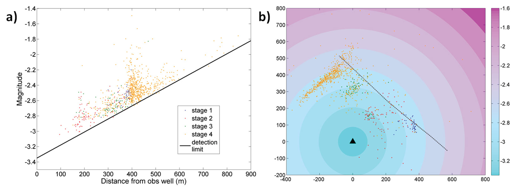
In order to determine the detection threshold, magnitudes of events are plotted against distances between events and the observation well (Figure 8(a)). The detection slope equals 0.0017. Figure 8(b) shows the contour plot based on the inferred detection threshold with overlaid events for the four stages. Most recorded events for stages 1 to 3 spread towards the observation well and no events beyond the magnitude -2.6 contour line are mapped for these stages. This indicates a potential bias in the event cloud shape due to the detection threshold. Stage 4 created more events, and the cloud spreading transversely to the observation well, its shape is well defined and does not seem to be affected by the detection threshold on the left side of the treatment well. However much fewer events are mapped on the right side of the well, suggesting again a possible bias due to the detection limit. A minimum common magnitude threshold cannot be inferred from the magnitude-distance plot (Figure 8(a)), which is also an indication that the whole fracture was not mapped (Cipolla et al., 2011).

Dataset 2

The second dataset of microseismic events was also recorded during the hydraulic fracturing treatment of gas shales but in a different reservoir than dataset 1. Eight stages from the same treatment well are analyzed. The microseismic events for the first four stages were recorded using only a single observation well A (Figures 9(a)). In that particular case the detection slope reaches about 0.0004, much lower than for the previous dataset. This discrepancy is certainly due to different geology of the reservoir. The minimum common magnitude is equal to -3. The major axes of event clouds are oriented radially to the observation well (Figure 9(a)), but no clear asymmetry can be seen the event cloud shapes.

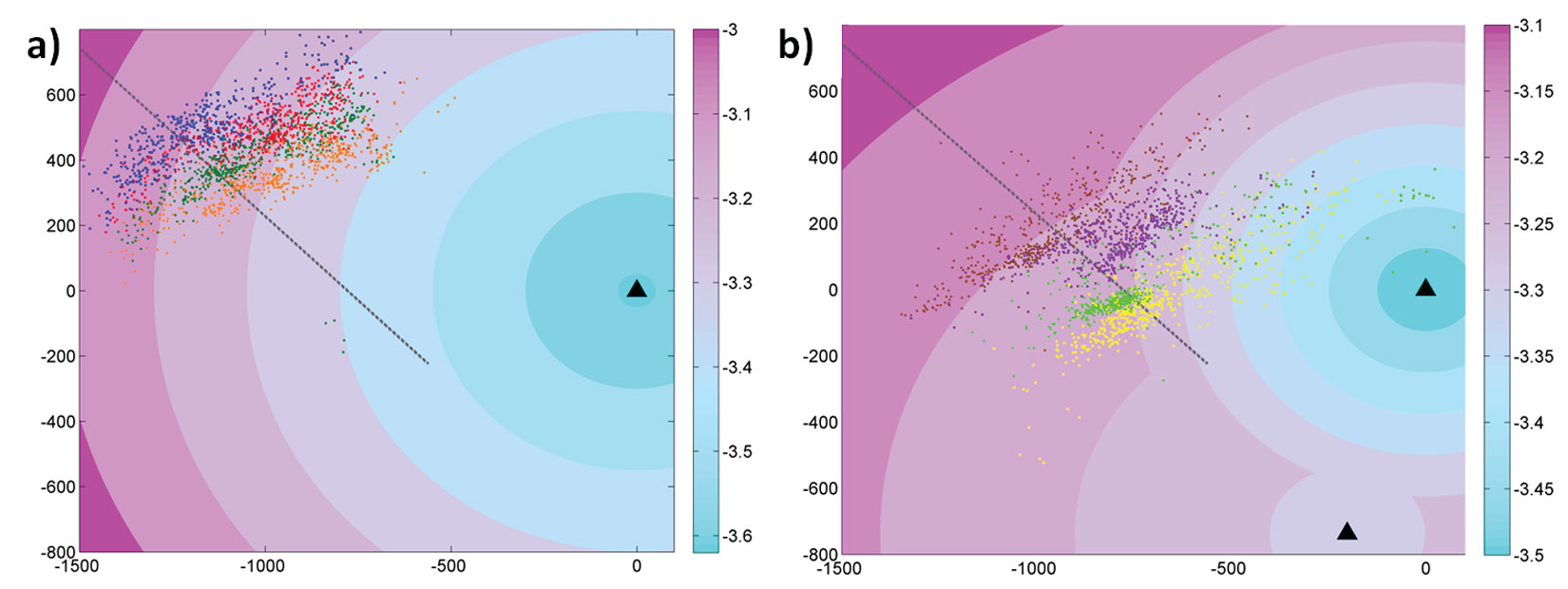
Stages 5 to 8 from the same horizontal treatment well were recorded using two observation wells A and B (Figure 9(b)). The detection slopes from observation wells A and B are respectively 0.0004 and 0.0001. The two different detection thresholds could indicate changes in the geology or could be due to different orientations of event clouds to both observation wells. Indeed event clouds are oriented rather radially to observation well A but transversely to observation well B. Microseismic events of stage 5 (brown dots) spread rather evenly on both sides of the treatment well and are thus not affected by the detection threshold. Most events of stage 6 (purple dots) are mapped on the right side of the treatment well, but this is certainly due to the mechanical behaviour of the reservoir as magnitude threshold is similar along the major axis of the event cloud for that stage. Event clouds for stages 7 and 8 spread quite far on both sides of the treatment well and are even a bit denser on the left side of it although the detection threshold is slightly higher on that side. This leads to the same conclusion as for the single observation well: the detection threshold slope is too low to introduce a real bias in the event clouds.

Using two monitoring wells in that particular case does not improve the interpretation of microseismic events.

Discussion

Some authors use the Gutenberg-Richter relationship to account for possible non-detected small events and then compare the reconstructed seismic energy with the total injected energy (Boroumand and Eaton, 2012; Maxwell et al., 2008). Our study demonstrates that the b-value is strongly influenced by the detection threshold. So the estimated b-value may be an under-estimation of the real b-value.

Isolated events in real datasets are often considered as outliers to the closest cloud of events and included in its statistical analysis. We showed that these isolated events could also simply belong to a cloud of events in which most of the events have a magnitude lower than the detection threshold and thus are not recorded (see especially clouds from well 3 in Figure 1). Williams and Calvez (2013) suggest a method to reconstruct part of the magnitude distribution to improve the b-value estimation and help the interpretation.

Other factors not mentioned in this work could affect the shape of event clouds such as signal to noise ratio, uncertainty in event locations, anisotropy due to geological features or radiation patterns linked to failure mechanisms (Cipolla et al., 2011; Zimmer, 2011). If using our method to plan an acquisition geometry, those factors will have to be included in the computation of the detection threshold.

Conclusions

The radial orientation of the event clouds and the slope of the magnitude-distance threshold are the dominant parameters influencing the asymmetry of event clouds further from the observation well. The frequency-magnitude parameter b changes significantly and variances of that parameter increases drastically with increasing detection threshold, thus leading to less accurate values of b. Care must be taken when trying to use these variations for interpretation as they may result from detection deficiency. Recording events with two observation wells helps limiting the influence of the detection threshold and ensures the overall shape of the microseismic event clouds is captured. Despite its simplicity the simulations presented above are a useful tool to qualify and quantify the loss of information linked to a chosen acquisition geometry.

Acknowledgements

The authors thank the Microseismic Industry Consortium for funding. They are grateful to ConocoPhillips and EOG Resources for providing data.