Introduction
Hydraulic fracture stimulations or ‘fracs’ are vital for economic production in low permeability tight gas and shale gas reservoirs, and the frac height is a key factor for engineers to optimize the hydraulic fracture treatment. As unconventional reservoir development has spread through North America and specifically to regions unaccustomed to petroleum production, public awareness of hydraulic fracturing has increased. Environmental concerns have also grown, including protection of shallow freshwater aquifers. Fortunately within the engineering and geophysical literature there are a number of published microseismic results in numerous settings and various depths. These examples shed light on the factors that control height growth, and show the actual hydraulic fracture heights that are created in a variety of reservoirs.
Hydraulic fracturing involves fluid injection at sufficient pressure to create a tensile fracture in the formation, which will tend to grow perpendicular to the minimum stress direction. At the depths of most petroleum reservoirs, the minimum stress is approximately horizontal, which results in the creation of a vertical fracture. The vertical fracture height growth is of interest for various engineering reasons, particularly related to coverage of the reservoir depth range and outof- zone fracture growth. Hydraulic fracture engineers have developed modeling tools to enable prediction and simulation of frac geometry, including the fracture height. The creation of these engineering tools has also spawned a need for fracture imaging technologies to monitor and validate fracture growth. Several techniques exist, including tracers, distributed temperature and vibration sensors that monitor near-wellbore fracture geometry. However, in order to monitor the hydraulic fracture growth away from the wellbore microseismic monitoring has proven to be the most valuable technology.
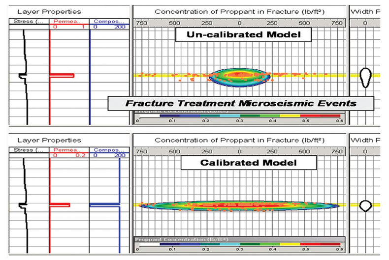
In the early days of hydraulic fracture simulation, the fractures were modeled as simplistic penny shaped cracks in infinite elastic media. These models tend to estimate approximately circular fractures, as tall as they are long. More advanced approximations were able to account for depth varying material properties and ultimately the associated variable stresses. As monitoring technologies began to provide insight into the actual growth, evidence quickly mounted that fracs are not as simple as initially thought. 2D hydraulic fracture models have been available for quite some time, and have evolved in order to better match observed fracture geometries. As an example, consider the application to a project which included microseismic data (Figure 1). Typically these fracture models match injected pressures and net volumes (include fluid leakoff from the fracture) to hydraulically model the resulting fracture profile. The mechanical material properties and stresses are also used to geomechanically constrain the hydraulic fracture mechanics. In this example, the initial modeling (top of Figure 1) incorporated stress and material property variations around a thin reservoir, and predicted some fracture containment within the reservoir. This ‘uncalibrated’ model predicted both upward and downward growth which limited the length of the fracture. However, the microseismic monitoring results (overlain on both models) showed that the fractures were contained entirely in the reservoir and that the actual fracture length was much longer than originally anticipated. The microseismic data was used to ‘calibrate’ the model (bottom of Figure 1), by adjusting the input parameters such that the predicted and observed geometries match. The fracture model also predicts the proppant concentration in the fracture (contours) that will define the relative permeability enhancement associated with the fracture. In this example the calibrated model predicts a geometry that is more favorable from a reservoir contact point of view, since the depth containment results in a longer fracture mostly in the reservoir with little out-of-zone fracturing. In order to match the microseismic geometry an additional material property of composite layering was included as shown by the blue track on the left side of Figure 1. This composite layering (or its equivalent) has found its way into many fracture simulation workflows and has proven to be an important factor to match the fracture containment that is typically observed.
Geology Controls on Fracture Growth
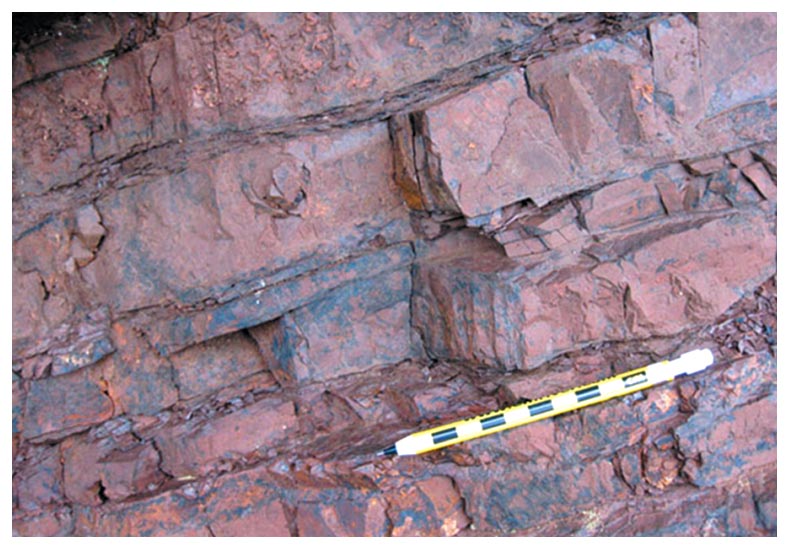
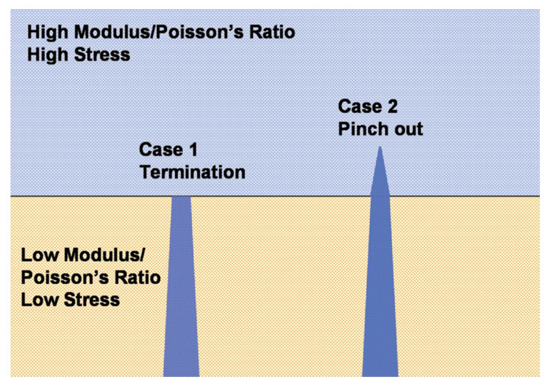
In order to understand this composite layering effect, it is informative to examine geologic examples of fracture growth. Figure 2 is a downloaded geologic section with annotated fractures. Notice that all of the fractures eventually stop at a bed boundary. Some fractures persist longer than others and cross some bedding planes but all eventually terminate. Figure 3 highlights one potential cause of the bed termination. This example illustrates that the containment is related to changes in the fabric of the rock and can be caused by thin laminations between thicker layers. Consider possible causes as shown in Figure 4 depicting two alternate views or end members of the possible effect of fractures growing between layers with different properties. The layering could correspond to fractures growing from a soft shale unit into more brittle layers (a common lithologic section in many shale gas reservoirs surrounded by limestone layers). Horizontal stresses will tend to be amplified in the stiffer layers associated with the increased load bearing capabilities. Increased stress will tend to limit fracture growth for similar fracture pressures, due to a lower net pressure acting on the fracture face. In addition, fractures in the stiffer rocks will open less for a given pressure increase, limiting their ability to accommodate fluid. Together the stress and compressibility define geomechanical conditions that tend to restrict hydraulic fracture height growth. The alternate scenario depicted in Figure 4 involves the fracture completely terminating at the interface. (Note that variations between these two scenarios are also possible including fracture ‘offsets’ or deflection where the frac partially grows along the interface layer). If the bedding plane is mechanically weak and allows the two layers to move independently, the fracture opening in one layer may not translate to fracture opening in the second layer. If the bedding plane is either not welded or contains thin laminations (such as Figure 3) the associated VTI strength anisotropy may hinder the fracture crossing the interface. Instead the fracture may either terminate or grow along the interface depending on the geomechanical and hydrodynamic conditions. Bedding laminations are analogous to automobile safety glass structure, where laminated layers of glass are used to limit fracturing entirely through windshields (as known by many of us Alberta drivers watching fractures grow from stone chips!). Composite layering in rocks tends to limit the overall hydraulic fracture height growth, and fracture simulations have found these to be an equally important factor together with geomechanical variations. The combined impact of these factors limits fracture height growth, both for natural and hydraulically created fractures.

Limited fracture height growth can impact the ability of a single horizontal well to contact a thick reservoirs section, resulting in engineering challenges to drain the reservoir with few horizontal wells. Consider an example from the Montney. Depending on the location there could be a thick potential target zone spanning from the Lower to Upper Montney and in places up into the overlying Doig. Figure 5 shows microseismic data recorded while fracing a horizontal well targeting the Upper Montney. In this case, the microseismicity shows that the frac was successfully contained within the Upper Montney (a few events locate in the Doig but are attributed to location resolution) and that relatively long horizontal fracture wings were created providing good reservoir contact area. In this case the Upper Montney is the target and so the fracture containment is favourable, but for discussion purposes consider a hypothetical example where the intention is to create a hydraulic fracture that grows upwards and downwards. In these conditions, it would be an engineering challenge to contact a large depth interval which could be overcome by modifying the fracture injection parameters (often injection rate is the control) or changing the horizontal well landing point and drilling the well at a different depth. In the Horn River for example, microseismic monitoring is being used by various operators to look at containment in the Muskwa and Evie shales in order to understand the depth containment and interactions between wells drilled into the different layers.
How can geophysics help? Clearly the engineers want to be able to characterize the geology sufficiently to robustly predict containment. There is a lot of effort being made to extract stresses and rock properties from seismic reservoir characterization to help quantify hydraulic fracture response and define sweet spots. While sweet spot identification is an important aspect for well placement, in terms of height containment thinly laminated beds such as shown in Figure 3 may occur below seismic resolution. Ultimately robust geomechanical characterization will likely require an integrated approach of geology and geophysics, including high resolution wireline measurements of sonic and formation imaging. We face technical challenges as we travel this path: such as up-scaling between log and seismic and extrapolating from high resolution well based imaging. To help bridge this gap, microseismic is the key technology to validate and confirm the geomechanical earth model. Imaging height growth and validating the fracture containment characteristics is an important engineering application of microseismic and one of the reasons that microseismic is an important component in the both the appraisal and development phases of unconventional resources. Microseismic provides insight into a number of aspects of the hydraulic fractures, but in particular has opened the engineer’s eyes to issues of height containment as discussed earlier. Extensive industry knowledge has been built from tens of thousand of fracs that have been imaged using microseismicity. While the results of all this monitoring are obviously proprietary to the individual operators, it has provided insight into fracture growth as well as competitive advantages around the best fracing practices for a given reservoir.

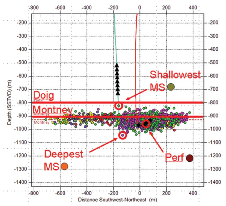
As the search continues to predict fracture containment, a large number of papers have been written showing the microseismically imaged hydraulic fracture growth in many unconventional reservoirs. These publications provide released examples of the microseismic hydraulic fracture height (number of publications is too large to provide a complete listing of the papers here). For each published example the depth of the upper and lower most microseismic event and associated average perforation depth was determined as illustrated in Figure 5. In some cases, multiple stages of a given project were included in the publication but here only a representative example is included intentionally using the example with the largest height growth. Figure 6 shows a plot of the depth to the shallowest microseism, perforation (frac initiation depth) and deepest microseism. Several well known reservoirs have been highlighted: including examples of the Montney, Horn River and Cardium. Perforation depths vary between about 1200 to 3500 m, although for each of the reservoirs there will be a variety of perforation depths beyond that flagged in this plot. Note that while there is a large variation in the height growth from project to project the top of the hydraulic fracture tends to get deeper as the well or frac initiation gets deeper. Figure 7 shows the relative upward and downward growth to better illustrate the variation. Notice that there tends to be more upward growth than downward growth, which does not appear to be a detection bias. The most probable explanation is that stress tends to decrease upward, favouring upward growth into lower stress rocks which is accentuated by frac fluid buoyancy effects. Also note that significant upward growth is limited to a few cases and most examples tend to be less than about 100 m. Figure 7 also shows the average upward and downward height along with a histogram, which is summarized in the table below.
| Upward Growth | Downward Growth | |
|---|---|---|
| Table 1. Statistics of the data depicted in Figures 6 and 7. | ||
| Mean +/- stand dev | 80 m +/- 87 m | 73 m +/- 48 m |
| Maximum | 295 m | 190 m |
| Minimum | 12 m | 10 m |

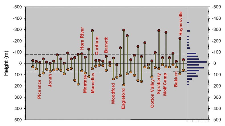
The variation in height growth between locations is expected with the variation in injection rates, geomechanical variations and reservoir settings depicted in this broad sampling. Within a given setting, the overall height growth tends to be fairly consistent with the examples included here. For example, in the Haynesville and Wolfcamp/Spraberry upward fracture growth tends to be commonplace, while in formations such as the Cardium sands hydraulic fractures are often vertically contained. The height growth summarized here also provides context regarding concerns around the possibility of fracing into aquifers. While the depth to the bottom of an aquifer depends on the geographical location, most tend to be relatively shallow. The average top of the fracs shown here is more than 2 km below the surface much deeper than freshwater aquifers. The data shows a significant thick buffer of rock above the top of the hydraulic fracture. Obviously in particular cases where there may be a shallow frac or regions with particularly deep aquifers, targeted monitoring may be advisable to ensure aquifer integrity.
Conclusion
In conclusion, examples of hydraulic fractures in many different reservoirs demonstrate contained height growth which is directly analogous with natural fractures. As fractures grow vertically and pass through different lithologies, the geomechanical conditions change and limit height growth. Composite horizontal layering also imposes additional height containment. From an engineering perspective contained hydraulic fracture height growth can be either good or bad news. In thin reservoir targets, containment favours longer fractures and increased reservoir contact area, whereas in thick or layered reservoir targets, containment can introduce challenges associated with contacting the entire reservoir depth interval. Ultimately this may lead to having to use multiple horizontal wells at different depths to drain the entire target interval. However, containment is good news from an environmental perspective, because it results in limited hydraulic fracture height growth and an associated buffer between deep fractures and shallow aquifers.

Related Reading


Join the Conversation
Interested in starting, or contributing to a conversation about an article or issue of the RECORDER? Join our CSEG LinkedIn Group.
Share This Article