AVO attributes of gradient and intercept are related to the reservoir properties based on rock physics knowledge. We develop a new rock physics model based inversion method in this study where we apply the Xu-White shaly-sand mixture model and simultaneously invert the reservoir properties of clay content, water saturation, and porosity with standard deviations from AVO attributes. The method is applied to the seismic data of the Gulf of Mexico at two areas: King Kong and Lisa Anne. After inversion, the fizz and gas reservoirs are differentiated for King Kong and Lisa Anne.
Introduction
Conventionally, the reservoir properties can be inverted first by doing the impedance inversion (P-impedance, S-impedance, or Elastic Impedance inversion) and second by deriving the reservoir properties using the rock physics relationship calibrated from the well. Li et al. (2005) inverted porosity and water saturation from AVO attributes. Chi and Han (2007a and 2007b) inverted reservoir properties from AVO attributes and also developed a method to differentiate fizz and gas reservoirs based on AVO inversion. In this study, we invert reservoir porosity, water saturation, and shale volume with standard deviations directly from seismic AVO attributes.
The rock physics model in this inversion is the Xu-White shaly-sand mixture model (Xu and White, 1995 and 1996; keys and Xu, 2002). The mathematical expressions contained within the shaly-sand mixture model provide a method for determining P-wave velocity, S-wave velocity, and density of the sub-surface rock given shale volume, porosity, and fluid properties as well as properties of minerals and their pore aspect ratios. In this rock physics model, the porosity is incrementally increased by using the differential effective medium theory. After the dry elastic properties are estimated, the bulk modulus and shear modulus of the saturated rock are calculated by using the Gassmann’s equation. Then the P-wave velocity, S-wave velocity, and density can be calculated for the saturated rock.
The posterior probability can be written as
P(Cj|Attributes) = k x P(Attributes|Cj ) x P(Cj ),
where Cj is the water saturation, porosity, and shale volume, Attributes are the intercept and gradient, P(Cj ) is the probability density function for Cj , and P(Attributes | Cj ) is the conditional probability of Attributes given Cj . The posterior probability P(Cj|Attributes) is calculated as the combination of the prior probability function, the likelihood function, and the normalization coefficient k . When P(Cj ) has an uniform distribution, the posterior probability is directly proportional to the likelihood function.
The forward modeling
A two half-space model is constructed to test the effects of porosity, water saturation, and shale volume on intercept and gradient. The top space in the model is shale and the bottom one is sand. Given sand and shale properties in the model, the intercept and gradient can be calculated in different incident angles. The shale properties are the averaged values of well logs in shale segment and the sand properties are calculated in forward modeling based on the shaly-sand mixture model. For the sand, the porosity is from 0.1 to 0.4, the shale volume is from 0 to 0.3, and the water saturation is from 0 to 0.9. In this study, it is assumed that porosity, shale volume and water saturation vary independently.
The parameters used in the modeling shown in the following tables:
| P-velocity (km/s) | S-velocity (km/s) | Density (g/cc) | |
|---|---|---|---|
| Table 1. The parameters of top shale | |||
| Shale | 2.59 | 1.10 | 2.33 |
| Shale | Sand | ||
|---|---|---|---|
| Table 2. Pore aspect ratios of shale and sand | |||
| Pore aspect ratio | 0.04 | 0.15 | |
In the forward modeling, the porosity, water saturation, and shale volume of the sand are varying at the same time. Since the P-wave velocity, S-wave velocity, and density of the sand change with porosity, water saturation, and shale volume in forward modeling, the calculated intercept and gradient are the functions of porosity, water saturation, and shale volume.
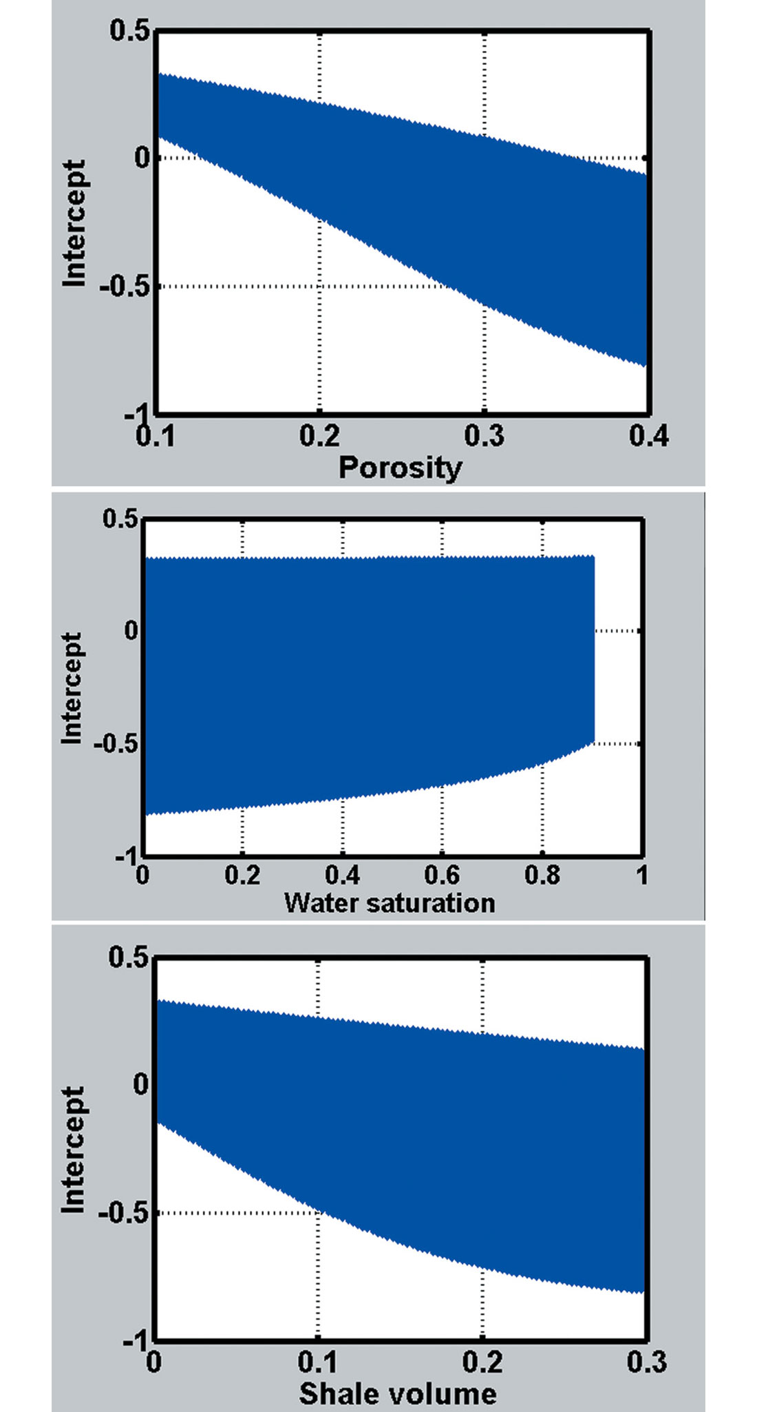
(a) projection of intercept on porosity axis
(b) Projection of intercept on water saturation axis
(c) Projection of intercept on shale volume axis
Figure 1 shows that results of intercept as function of porosity, water saturation, and shale volume, which are combined randomly in forward modeling. Figure 1a is the projection of intercept on porosity axis, Figure 1b is the projection of intercept on water saturation axis, and Figure 1c is the projection of intercept on shale volume. For instance, if there are no variations of water saturation and shale volume in Figure 1a, there will be a single line to show intercept decreases with increasing porosity. Based on Figure1, the intercept decreases when increasing porosity or shale volume and increases when increasing water saturation.
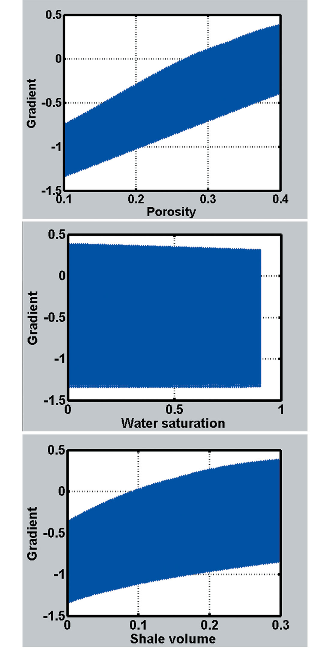
(a) projection of gradient on porosity axis
(b) Projection of gradient on water saturation axis
(c) Projection of gradient on shale volume axis
Figure 2 shows that results of gradient after drawing porosity, water saturation, and shale volume randomly in forward modeling, which is similar to Figure 1. Based on Figure 2, the gradient increases when increasing porosity or shale volume and decreases when increasing water saturation.
The conditional probability
The conditional probability describes the probability for intercept or gradient given certain conditions of porosity, shale volume, and water saturation. In this inversion procedure, the conditional probability is derived from stochastic modeling and combined with the prior probability to calculate the posterior probability for reservoir properties.
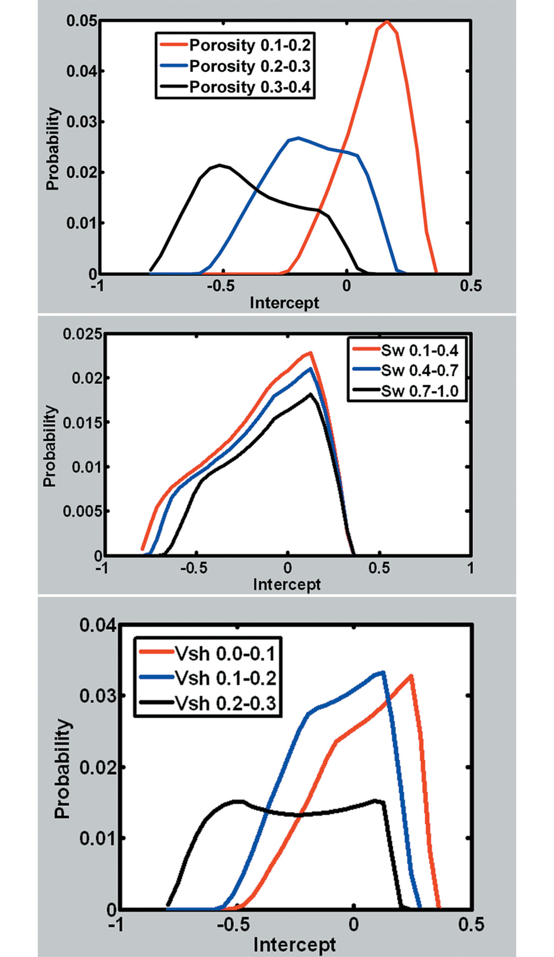
(a) The conditional probability given range of porosity
(b) The conditional probability given water saturation
(c) The conditional probability given range of shale volume
Figure 3 shows the probability of intercept given three ranges of porosity, water saturation, or shale volume. The red curve represents the smallest range and the black curve represents the largest range. The blue curve is in the middle range. Figure 3a shows the intercept decreases with increasing porosity and the intercept has higher probability in the lower range of porosity. Figures 3b and 3c show that the intercept has the lower probability when water saturation and shale volume are in the higher ranges.
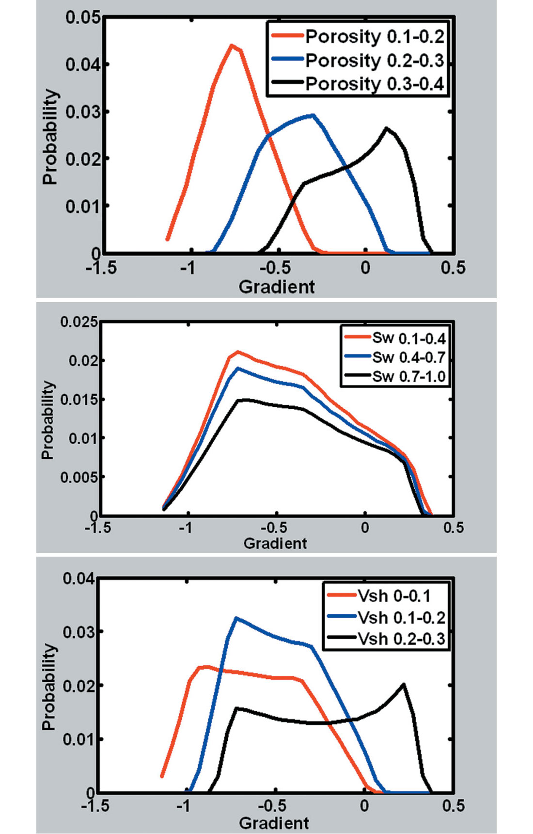
(a) The conditional probability of gradient given range of porosity
(b) The conditional probability of gradient given range of water saturation
(c) The conditional probability of gradient given range of shale volume
Figure 4 shows the probability of gradient given three ranges of porosity, water saturation, or shale volume, which is similar to Figure 3. Figure 4a shows the gradient increases with increasing porosity and the gradient has higher probability in the lower range of porosity. Figures 4b and 4c show that the gradient has the lower probability when water saturation and shale volume are in the higher ranges.
The case study
In this study, we utilize seismic datasets acquired from King Kong and Lisa Anne in the deepwater Gulf of Mexico. King Kong is located in the western flank of a minibasin controlled by the underlying salt body while Lisa Anne is located in the southeastern flank (O’Brien, 2004). The targets in both of the two fields are unconsolidated sand reservoirs. The top and bottom layers are shale.
In this study, we assume that King Kong is drilled, Lisa Anne is not drilled, and the target reservoirs of King Kong and Lisa Anne have similar thickness. Thus, we can estimate the porosity, water saturation, and shale volume for King Kong after drilling and predict them for Lisa Anne before drilling.
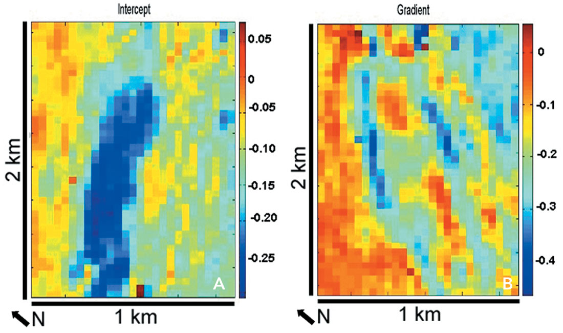
(a) The intercept of King Kong
(b) The gradient of King Kong
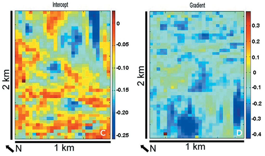
(c) The intercept of Lisa Anne
(d) The gradient of Lisa Anne
Figure 5 shows the intercept and gradient which are derived from the seismic angle gathers at King Kong and Lisa Anne. The King Kong well logs are used to calibrate the derived intercept and gradient.
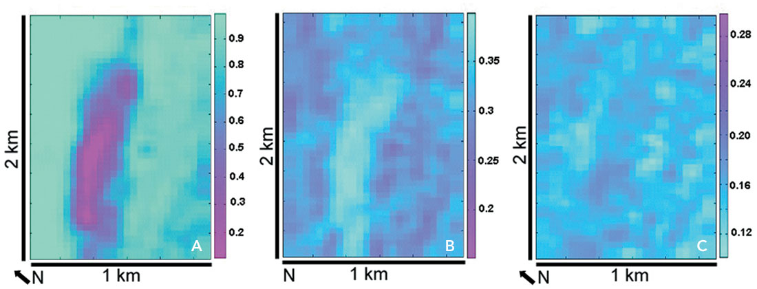
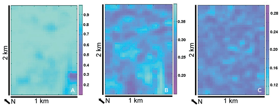
(a) Water saturation
(b) Porosity
(c) Shale volume
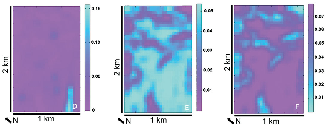
(d) Standard deviation of water saturation
(e) Standard deviation of porosity
(f) Standard deviation of shale volume
After the inversion, the final estimations and standard deviations of porosity, water saturation, and shale volume for King Kong are plotted in Figure 6.
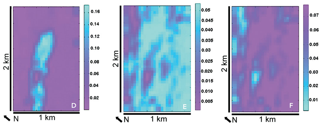
(a) Water saturation
(b) Porosity
(c) Shale volume
(d) Standard deviation of water saturation
(e) Standard deviation of porosity
(f) Standard deviation of shale volume
After the inversion, the final predictions and standard deviations of porosity, water saturation, and shale volume for Lisa Anne are plotted in Figure 7.
After inversion, the distribution of gas-saturated zone at King Kong is estimated and the fluid property of Lisa Anne is predicted. The inversion results show that King Kong is gas-saturated and Lisa Anne is fizz-saturated. The porosity and shale volume are simultaneously inverted with water saturation for King Kong and Lisa Anne. The inverted results of King Kong and Lisa Anne are consistent with drilling results. The standard deviations show the estimation and prediction confidence for the inversion results. The water saturation has higher standard deviation than the porosity and shale volume.
Conclusions
In this study, the shaly-sand mixture model based inversion method is applied to the seismic data of the Gulf of Mexico. We simultaneously invert water saturation, shale volume, and porosity for the reservoirs of King Kong and Lisa Anne based on the fact that AVO attribute are related to rock properties. The inversion results show the distribution of water saturation, shale volume and porosity for King Kong and the prediction of water saturation, shale volume and porosity for Lisa Anne. The predicted fizz saturation at Lisa Anne is consistent with drilling result. This inversion procedure is a practical way which can be applied to other areas to differentiate fizz and gas reservoir and predict reservoir properties.

Acknowledgements
We wish to thank sponsors of UH/CSM Fluid/DHI consortium for their supports. We also thank Anadarko Petroleum and WesternGeco for permission to show the seismic data.


Join the Conversation
Interested in starting, or contributing to a conversation about an article or issue of the RECORDER? Join our CSEG LinkedIn Group.
Share This Article