For decades passive seismic monitoring has been a routinely used tool in earthquake engineering, mining and geothermal industries. In the past 10 years its use in the petroleum industry has seen an order of magnitude growth: in terms of annual revenue the global market is now more than a ¼ billion USD. Most of this growth has been stimulated by the rapidly developing shale gas sector, where microseismic technology is used to monitor hydraulic fracture stimulation.
The primary purpose of microseismic monitoring during shale gas stimulation is to locate events to estimate the stimulated reservoir volume. This can be done using borehole arrays of three-component geophones or surface arrays of sensors, each approach having its advantages and disadvantages. More recently the broader potential for using microseismic data to image the reservoir has been considered. For example, anisotropy is a seismic attribute that is well suited to being studied using either small naturally occurring or stimulated earthquakes. Such events are effective in generating shear-wave energy and are therefore well suited to shear-wave splitting analysis – arguably the least ambiguous indicator of anisotropy. This splitting may be due to the intrinsic anisotropy of the rock or it may be an indicator of aligned fracture or crack sets (provided the fracture/crack spacing and size is much smaller than that of the dominant seismic wavelength; Crampin, 1984). Here we discuss how down-hole recordings of shear-wave splitting can be used to image fracture-induced seismic anisotropy.
Microseismic datasets are generally large, with many 1000s of events commonly recorded. Therefore shear-wave splitting analysis must be automated in its execution. With sufficient data coverage and an assumed model for the cause of anisotropy, the splitting measurements can be then inverted for a range of anisotropy mechanisms. At its simplest this may be anisotropy due to a single set of vertical fractures, which leads to a horizontal transverse isotropy (HTI). This constrains a range of fracture characteristics, including fracture strike, density and compliance. If the anisotropy is observed to be frequency- dependent, the poroelastic properties of the medium, as well as the dimensions of fracture sets, can be estimated. Cumulatively, such anisotropy analysis can provide useful information for assessing the efficacy of hydraulic fracture stimulation, but also provides a useful probe of naturally occurring fractures in a range of reservoir settings.
Automated shear-wave splitting analysis
A characteristic of wave propagation in anisotropic media is the propagation of two independent shear waves. When a shear-wave (e.g., generated by an earthquake) travels through an anisotropic medium it ‘splits’ into two orthogonally polarised shear-waves that have different seismic velocities (Figure 1). The two shear-waves separate over the length of the ray path and the time delay (δτ) between the two shear-waves is proportional to the magnitude of the anisotropy and the ray path length. The polarisations of the fast (φ) and slow shear-waves are indicators of the anisotropic symmetry of the medium. Measurements of these two splitting parameters (δτ and φ), coupled with observations for a range of propagation directions, can be used to characterise the anisotropy.
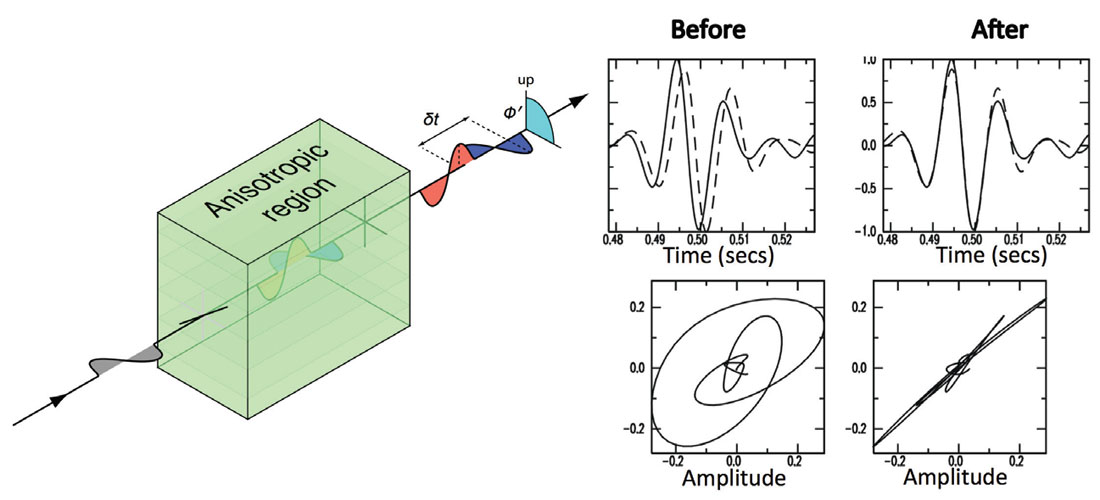
Shear-wave splitting analysis is now a routine tool in earthquake seismology (e.g., Savage, 1999). A common approach is to work in ray centred coordinates and then rotate the two components perpendicular to the ray direction by φ and shift their relative time by δτ. This removes the effect of the anisotropy (i.e., the splitting) and linearises the particle motion (Figure 1). Mathematically this can be described as minimizing the second eigenvalue of the covariance matrix in a predefined window of time around the shear-wave arrival (Silver and Chan, 1991). Another popular approach uses waveform cross-correlation to find the δτ and φ that best isolates the fast and slow shear-waves (e.g., Menke and Levin, 2003).
Passive seismic monitoring of a reservoir will routinely record many 1000s of events and manual analysis of shear-wave splitting is therefore impractical. Teanby et al. (2004a) and Wuestefeld et al. (2010) developed a semi-automated workflow for estimating shear-wave splitting using S-wave travel-time picks and a cluster analysis to assess the robustness of the solutions. Furthermore, the methodology of Wuestefeld et al. (2010) uses both the eigenvalue method and the cross-correlation method to formulate a quality factor, which effectively provides a robust estimate of the reliability of splitting measurements. Filtering and error analysis provides further steps to identify truly unique results. Typically only 10-20% of the sourcereceiver combinations in a given dataset produce reliable results, with noise and unfavourable ray directions usually being responsible for the unreliable measurements. Nevertheless, as the datasets are normally very large, a large number of splitting parameters can be routinely obtained.
Evidence of shear-wave splitting in microseismic datasets has been documented in a number of reservoirs. These include: North Sea chalk reservoirs (Valhall (Teanby et al., 2004b; de Meersman et al., 2009) and Ekofisk (Jones et al., in press, 2014)); carbonate reservoirs in west-central Oman (Al-Anboori and Kendall, 2010; Al-Harrasi et al., 2010) and southern Saskatchewan (Weyburn) (Verdon et al., 2011a); the tight siliciclastic reservoir of Cotton Valley in Carthage, Texas (Wuestefeld et al., 2011a; Verdon and Wuestefeld, 2013); a tight-gas sandstone (Baird et al., 2013); and geothermal reservoirs (e.g., Elkibbi and Rial, 2005).
Fracture inversion
Microseismic data acquired by borehole sensors are ideally suited to the study of seismic anisotropy. Unlike conventional reflection seismology, raypaths are not generally sub-vertical and hence directional variations in velocity are more easily assessed. Hence, shear-wave splitting measurements in boreholes can be used to assess fracture properties, which are sensitive to spatial and temporal variations in the stress field (e.g., Teanby et al., 2004b; Al-Harrasi et al., 2010; Verdon and Wuestefeld, 2013).
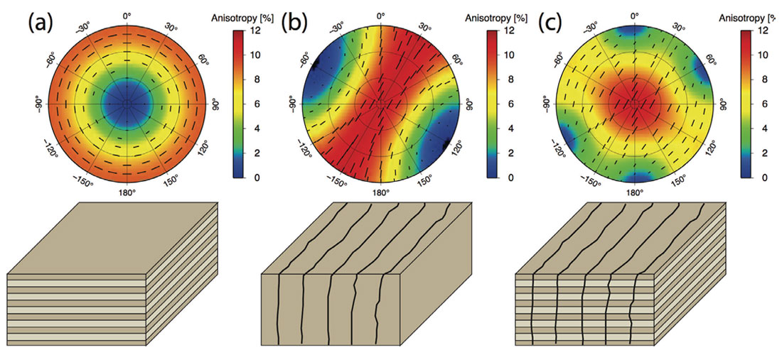
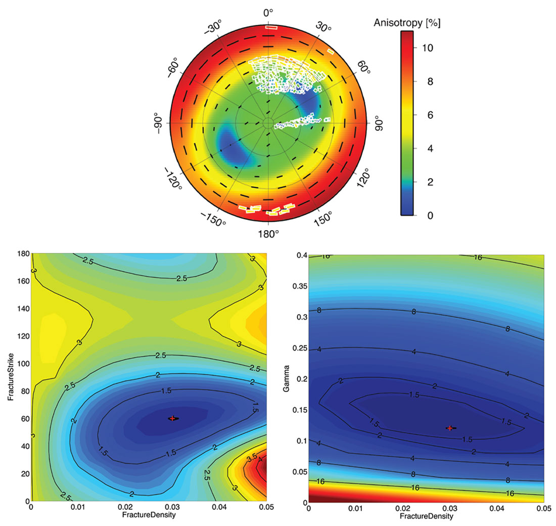
As mentioned, shear-waves are sensitive to fracture-induced anisotropy and as such can be inverted for fracture parameters. However, the challenge lies in separating fracture effects from other anisotropy effects, such as the intrinsic anisotropy of the host rock (e.g., Vernik and Liu, 1997; Kendall et al., 2007). Figure 2 shows how shear-wave splitting varies in style depending on the cause of the anisotropy. Verdon et al. (2009) outlined an inversion approach that uses rock physics modelling to select the best-fit fracture geometries and sedimentary fabrics to match shear-wave splitting observations. It should be noted that this only constrains the shearwave anisotropy, but P-wave information could be added to further characterise the anisotropy (see, e.g., Grechka and Yaskevich, 2013). The approach has been demonstrated using a passive seismic dataset collected during hydraulic fracture stimulation (Verdon et al., 2010). Figure 3 shows an example using data from monitoring tight-gas stimulation in east Texas using two wells (Wuestefeld et al., 2011a). The inversion successfully recovers fracture strike, fracture density and Thomsen’s (1986) γ parameter. Tests with synthetic data show that the success of these inversions is highly dependent on the range of arrival azimuths and inclinations that are available. It is therefore possible to determine in advance which structures are detectable with shearwave splitting, and which are not. This means that survey design can be used to identify potential trade-offs between parameters than can affect the accuracy of such inversions.
Verdon and Kendall (2011) generalized the inversion to detect the presence of two fracture sets. With one dataset, their analysis revealed a set of conjugate fractures that allowed CO2 migration through a carbonate reservoir (the Weyburn-Midale field). In contrast, a second dataset from a shale-gas environment revealed a single fracture set, stimulated through hydraulic injection.
Temporal variations in shear-wave splitting have been observed in a number of datasets, including those acquired in volcanic settings (Volti and Crampin, 2003; Gerst and Savage, 2004), mining settings (Wuestefeld et al., 2011b), producing oil reservoirs (Teanby et al., 2004b), and during hydraulic stimulation of tight-gas reservoirs (Wuestefeld et al., 2011a).
The magnitude of fracture-induced anisotropy is conventionally interpreted in terms of fracture density, however the influence of many other factors cannot be ruled out. For example, shear-wave splitting will be sensitive to fracture size and aspect ratio, the degree of fracture welding, fracture permeability, and fluid viscosity. For these reasons, Schoenberg and Sayers (1995) expressed the effective compliance tensor of the fractured rock as the sum of the compliance tensor of the unfractured background rock and the compliance tensors for each set of parallel fractures or aligned fractures. In this way no assumptions are made about the shape or connectivity of the fractures.
The notation B is commonly used to describe the compliance of an individual fracture, whilst Z is the tensor that describes the effective compliance of a set of fractures (e.g., Hobday and Worthington, 2012). The compliance matrix, Z, can be further decomposed into the compliance of the fractures to deformation normal to (ZN) and tangential to (ZT) the fracture face. Shear-wave splitting is very sensitive to the ratio of these compliances (ZN/ZT). In general, isolated fracture will show small compliance ratios and more connected fractures will yield larger ZN/ZT ratios. However, this is complicated by the effects of fluid viscosity and the dominant seismic frequency (see Table 1 and discussions in Verdon and Wuestefeld (2013) and Baird et al. (2013)).
| Low (→0) | ZN/ZT | High (→1) |
|---|---|---|
| Table 1. The dynamic fracture compliance ratio (ZN/ZT), which can be estimated from shear-wave splitting analysis, is sensitive to a number of parameters: the dominant frequency of the seismic wave; the viscosity of the fracture fluid; the permeability of the rock, including matrix and fractures; fracture cementation; and the bulk modulus of the fracture fluid. | ||
| High | Frequency | Low |
| High | Viscosity | Low |
| Low | Permeability | High |
| High | Cementation | Low |
| High | Fluid Bulk Modulus | Low |
As fluid ingresses into the formation, the permeability increases as fractures interconnect, leading to a rise in the ZN/ZT ratio. This may lead to a rotation in the polarization of the fast shear-waves propagating oblique to the fracture (e.g., Volti and Crampin, 2003; Gerst and Savage, 2004; Johnson and Savage, 2012; Baird et al., 2013), a less intuitive effect. Inverting for fracture compliance, Verdon and Wuestefeld (2013) and Baird et al. (2013) have shown temporal variations in shearwave splitting in tight gas reservoirs, which they attribute to the change in fracture compliance in response to hydraulic stimulation.
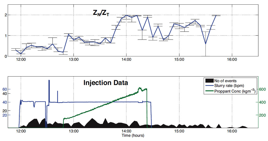
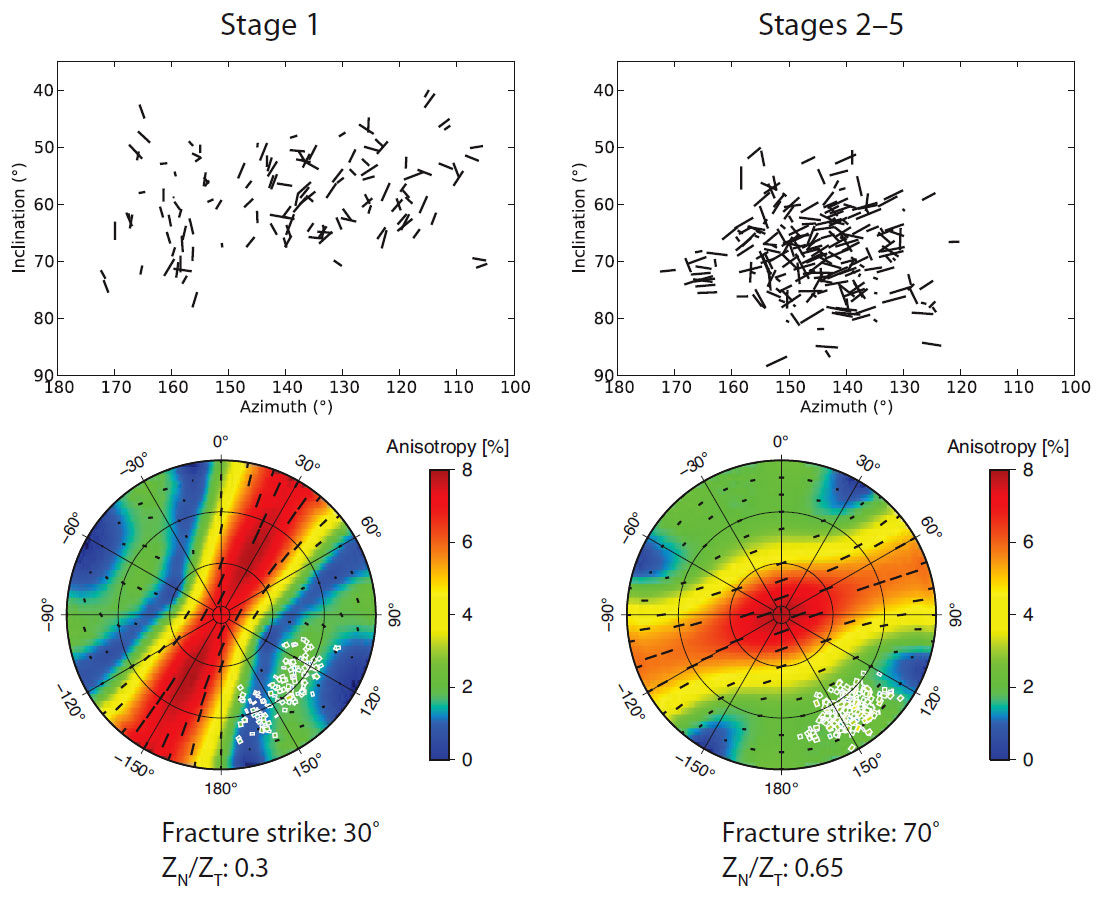
Figure 4 shows an example of how the ZN/ZT ratio varies with time during the stimulation of a tight gas formation (Verdon and Wuestefeld, 2013). The compliance ratio increases during the stimulation. This could be interpreted as the development of new fractures, the breakage of cement bonds in pre-existing fractures, or the improvement in connectivity between fractures (or all of the above). It is notable that the increase in fracture compliance ratio is coincident with the onset of proppant injection. Figure 5 shows examples of changes in shear-wave splitting and hence fracture properties between stages of a hydraulic fracture treatment. Baird et al. (2013) argue that pre-existing and partially welded fractures are initially dominant, but in later stages new fractures are stimulated parallel to the direction of maximum horizontal compressive stress. In both cases, splitting observed during the early stages of stimulation appears to represent existing, natural fracture networks. These networks have low ZN/ZT ratios, indicative of fractures that are poorly connected, and/or partially cemented. During the course of the stimulation, the compliance ratios of the fracture sets increase, implying that they are becoming better connected with each other and the rock matrix, and that welds and cement bonds in the fractures are being broken.
Frequency-dependent shear-wave splitting
In many reservoirs fracture orientation, density, size and connectivity control reservoir production. Work by Chapman and co-workers (e.g., Chapman, 2003; Maultzsch et al., 2003) has shown that the frequency dependence of shear-wave splitting can be very sensitive to these parameters. At low seismic frequencies a material with aligned inclusions will behave like a homogeneous anisotropic medium, but at higher frequencies the inclusions will behave as discrete scatterers. Poroelastic effects are more subtle. For example, aligned fluid filled fractures in a porous medium will exhibit frequency-dependent anisotropy. At high frequencies, the inclusions will be isolated and the effective anisotropy will be smaller, whereas at low frequencies, the inclusions are effectively interconnected and the anisotropy will be larger.
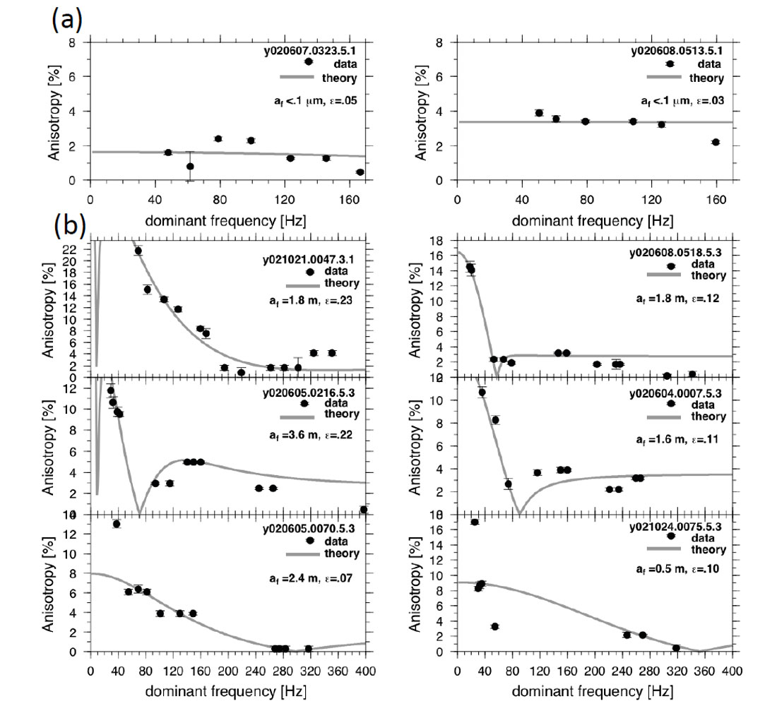
Borehole microseismic data are typically rich in frequency content, making them ideal for studies of frequency-dependent wave phenomena. The frequency content in datasets is somewhat variable with depth and lithology, but is generally between 10-400Hz. The analysis of frequency-dependent shear-wave splitting in microseismic data has been described in Al-Anboori and Kendall (2010) and Al-Harrasi et al. (2011). The data are filtered with overlapping passbands and the splitting parameters are then estimated for each frequency-band. The results presented in Figure 6 (from Al-Harrasi et al., 2011) reveal a lithology dependent variability in the nature of frequency-dependent shear-wave splitting. These results show large meter-scale fractures in the gas-producing carbonate reservoir and micrometer scale cracks in the sealing shale. These results agree with independent measures of crack/fracture size in this reservoir. Such analysis is ideally suited to detecting ‘sweet spots’ in tight gas reservoirs and monitoring fracture stimulation.
Conclusions and future directions
This paper has summarised recent research on deriving fracture properties from shearwave splitting measurements made on microseismic data acquired in a borehole. Shear-wave splitting analysis is easily automated, where the rate-limiting step is the speed of event location. Given sufficient ray coverage in azimuth and inclination, clusters of splitting measurements can be inverted for fracture properties such as density and orientation, including those for multiple fracture sets. Furthermore, these inversions can be used to track temporal variations in splitting, which are intimately related to variations in fracture density and fracture compliances. Early results suggest that these measurements may serve as a proxy for changes in permeability and fluid migration. Finally, the frequency dependent nature of shear-wave splitting is sensitive poroelastic effects and can be used to estimate fracture size.
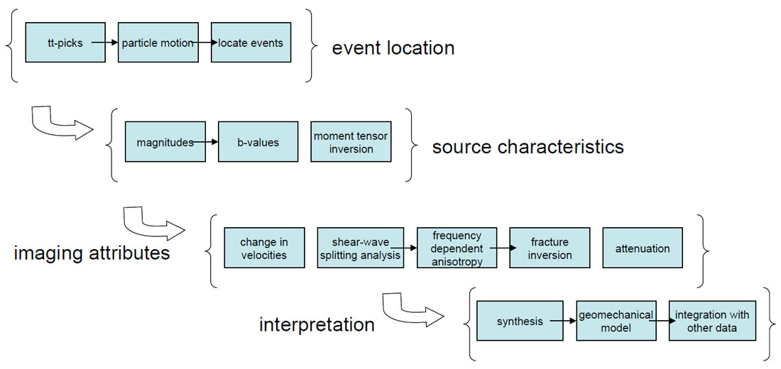
Splitting analysis is normally done as an afterthought in microseismic monitoring operation, and yet it holds potentially valuable information about fracture and crack properties. Figure 7 shows how this analysis can be routinely included in the workflow for analysing microseismic data. There are a number of potential applications of such anisotropy analysis both in passive seismic monitoring and monitoring hydraulic stimulations. Examples include: insights into the magnitude and orientation of the stress field, including hazardous stress build-up; helping determine anisotropy parameters for conventional seismic data processing; monitoring fracturing associated with injection fronts such as those due to water, CO2, and steam; a better understanding cap-rock leakage mechanisms and fault sealing; finally, post-mortem analyses of cases where hydraulic fracture stimulation has been unsuccessful.
Ideally, any monitoring operation would involve good baseline monitoring of seismicity. This could help better identify active faults, and potential fracture corridors as revealed through shear-wave splitting (e.g., Jones et al., 2014). The use of multiple borehole arrays of instruments helps to characterise the anisotropy with more certainty, but can also reveal spatial variations in anisotropy (e.g., Al-Harrasi et al., 2010). Finally, integration with surface seismic arrays or shallow borehole data would provide a more complete picture of anisotropy in the reservoir and overburden (e.g., Grechka and Yaskevich, 2013).

Acknowledgements
Funding for the work has been provided by the sponsors of the Bristol University Microseismicity Projects (BUMPS) and the Natural Environment Research Council (NERC), UK. James Verdon is a NERC Early-Career Research Fellow (Grant Number NE/I021497/1).


Join the Conversation
Interested in starting, or contributing to a conversation about an article or issue of the RECORDER? Join our CSEG LinkedIn Group.
Share This Article