Depth Imaging – “If We Could Turn Back Time”

Introduction

Seismic migration is an essential processing step in exploration plays involving any structural complexity, since migration is the process of placing seismic reflection energy in its proper subsurface location. The popular song “If I Could Turn Back Time” can describe the process of achieving accurate migration of seismic data through backward time propagation of wavefields.

In the process of imaging complex structures such as faults, and folds, we seek to reverse the path of surface-recorded seismic reflections back to the geologic reflectors. In essence, the idea is to “depropagate” seismic waves. The earliest geophysical publication on the use of complete wave equation solutions for reverse-time migration was presented by Hemon (1978) in a French paper entitled “Equations d’onde et modeles”. Hemon published the paper but did not believe it was practical. At about the same time, Dan Whitmore of Amoco Research was using the method extensively for the very practical problems of imaging overthrust structures and salt domes, but did not publicly disclose his results until participating in the 1982 SEG annual meeting’s migration workshop. Shortly thereafter, a number of papers on the subject appeared including independent research papers by Baysal et al (1983), Loewenthal and Mufti (1983), McMechan (1983), and Whitmore (1983). Baysal’s paper initiated the term “reverse-time migration” and gave some interesting overthrust examples. McMechan’s paper gave a lucid description of the algorithm’s simplicity and its generality. Subsequently, McMechan and his students have adapted reverse-time migration to almost every combination of migration problems including 2-D, 3-D, poststack, prestack, isotropic, and anisotropic situations. Whitmore et al. (1986) and Zhu and Lines (1998) showed how reverse-time migration compared to other popular depth imaging methods such as Kirchhoff and phase-shift migration. Mufti et al. (1996) showed that, with variable grids for finite-difference calculations, the method could be practically applied in three dimensions to the depth imaging of salt domes in Gulf Coast exploration.

Space and Time

Let us investigate the principles of reversing time in the migration process. Although some modern physicists will disagree, for all practical purposes we live in a four-dimensional world with three spatial dimensions plus the dimension of time. Any event that occurs is specified by its location in three-dimensional space and a specific time of occurrence. Physics deals with the fourdimensional space-time continuum. In space, we can go in forward or reverse directions. For example, in a 3-D Cartesian system we can travel north or south, east or west, up or down. However, with time in the physical world, we can progress only in one direction. We cannot physically go back in time and violate the principle of causality.

How is it possible, then, to perform reverse-time migration? To achieve this, we need to revisit the wave equation, which defines the propagation of seismic energy. Recall solutions to the wave equation for a 1-D homogeneous medium given by

D’Alembert showed that a general solution is of the form u=f(x+vt) + g(x-vt) where f and g are arbitrary functions which are twice differentiable. This can be shown by using the chain rule in partial differentiation and is derived in many books on the physics of waves including, for example, Becker (1954). It is fascinating that the solutions to the wave equation remain valid if we change the sign of t, the time variable. In other words the underlying physical processes of waves and the mathematical solutions to the wave equation remain unchanged if time is reversed.

Time-reversed Acoustics

This property of waves has led to the field of time-reversed acoustics as described in a recent Scientific American article (November 1999) by Mathias Fink, Director of the Waves and Acoustics Laboratory in Paris. At this laboratory, an array of microphones and speakers produces an acoustical “time-reversal” mirror. A speaker pronouncing a message “bonjour” to the mirror would receive the message “ruojnob” almost instantaneously converging back to the speaker’s mouth, as if the sound wave had experienced time reversal. This is achieved by microphones detecting the sound wave, passing the signal to a computer that stores the wave, reverses the signal, and sends it back along its original path. Although this may seem to be a somewhat comical experiment, it has many practical implications in the fields of seismic migration, underwater communication, materials testing, medicine, and seismic migration.

In medicine, for example, time-reversed acoustics can be used to break up kidney stones. Ultrasonic pulses from transducers bouncing off kidney stones can be focused back on the kidney stones causing them to break up. There are also research efforts into using the time-reversed acoustics method for the destruction of tumors. There are many useful and interesting applications described in Fink’s excellent Scientific American article, although the seismic applications are not mentioned. This missing item is unfortunate since seismic migration was probably one of the first successful applications of the method.

Reflection Seismology, Exploding Reflectors, And Reverse-Time Migration

In the simplest of terms, we can relate reflection seismology to reverse-time migration in terms of seismic wavefield propagation.

If we can imagine a movie showing wave propagation of reflected seismic energy, migration could be achieved by simply running the movie backwards so that seismic energy travels back to the reflectors from which it came. In a sense, migration indeed is the inverse of seismic wavefield modeling. A simple explanation for the zero-offset seismic experiment is given by Figure 1, which is taken from an AAPG Explorer article by Bording and Lines (2000).

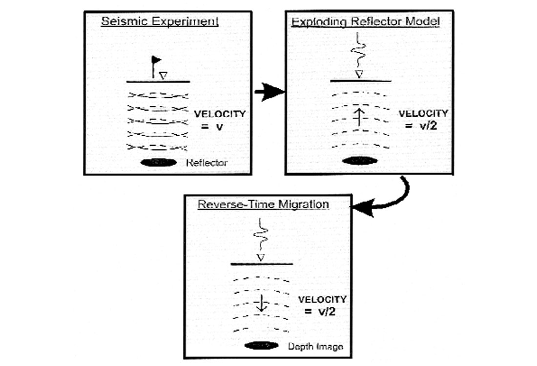
The reflection seismic experiment is shown in the upper left part of Figure 1 for a source and receiver at basically the same surface location. Seismic waves propagate with velocity v from a source (at the flag), down to a reflector, and then return back to a receiver (at the triangle). Dan Loewenthal pointed out that we can essentially view this experiment differently, in terms of an “exploding reflector” model, which is described in the upper right part of Figure 1. For most geometries, we can also think of the seismic response as being generated by seismic waves which travel a one-way path from “exploding reflectors” to the surface receivers (or half the distance) at a velocity that is half the true seismic velocity. This is a very useful concept for modeling since it generally gives a good approximation to a zero-offset section or to a stacked section, with considerably less compute time than computing the entire zero-offset section. It also helps us to understand depth imaging, since reverse-time migration processes the seismic data by reversing the path of the exploding reflector model as shown by the bottom part of Figure 1. The image is obtained by propagating the reflected energy backward in time with velocity v/2 to its point of origin (the reflector). For this discussion, we have dealt with the zero offset case of coincident sources and receivers - an approximation to the case of poststack migrations. Basically all the migration methods (reverse-time, Kirchhoff, phase-shift, finite-difference, etc.) have prestack versions which lend themselves to greater generality. We shall describe very briefly the imaging principle for prestack migration, referring the reader to Yilmaz (2001) for a discussion of the details of this important technology.

Loewenthal’s exploding reflector model allows us to think of a stacked section, which approximates a zero-offset section, in terms of the response to a set of reflectors that exploded at time zero. This thought experiment, in turn, allows us to formulate the migration problem as that of imaging the recorded wavefield at time zero, i.e., when and where the reflectors exploded. In fact, the exploding reflector model provides a very natural motivation for reverse-time migration (I have a section with positive times. How do I get the corresponding section inside the Earth at time zero? I have to propagate a wavefield with the arrow of time reserved!) Unfortunately, this model doesn’t tell us how to do prestack migration. Reflection inside the Earth takes place after the source has been excited but before the reflected energy has been recorded. So the time of reflection lies between time zero (the source time for a given shot) and the recording time for that event. If, at a particular location inside the Earth, we find the time when the wavefield from the source has passed through that location, we know that reflection has occurred there at that time. Then we must evaluate the recorded wavefield at the reflector location at the time of reflection. So prestack migration involves evaluating the wavefield from the source at all points inside the Earth at times greater than zero, the initiation time, and evaluating the wavefield from the receivers at all points inside the Earth at times less than the recording time. These operations are call downward continuations (in forward time from the source point and in reversed time for the receiver locations). Then the final image is built at each location from the downward-continued receiver wavefield at the instant that energy from the downward continued source wavefield strikes that point. Confused? Just think of Kirchhoff migration, which images a trace onto a reflector at time t_s + t_r, where t_s is the time from the source to the reflector and tr is the time from the receiver to the reflector. The first of these times expresses, in a sense, the downward continuation of the source wavefield, and the second expresses the downward continuation of the receiver wavefield. If these times are both stripped away, then both wavefields have been downward continued all the way to the reflector, and reflection occurs at time zero.

Example from the Canadian Foothills

The usefulness of “time-reversed acoustics” in depth imaging for foothills exploration can be demonstrated by examining some fault-fold models that are typical of the Canadian foothills. An example shown in Figure 2 requires the interpreter to distinguish between a fault-bend fold model and a fault propagation fold model.

Each model has been constructed using the GX Technology GXII software package. The total length of each model is 10 kilometers with a maximum depth of 4200 meters. Cell sizes are 10m by 10m. Velocities in Figure 2 are 2000 m/s (light gray), 2500 m/s (medium gray), 4000 m/s (dark gray) and 5500 m/s (black). All model parameters are equal. No topography has been included, layer thicknesses have been preserved, and the overall amount of structural shortening in each model is equivalent, therefore the only variable in each model and resulting image is the structural geometry.

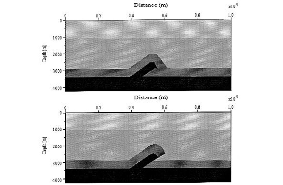
Although these models appear to be quite similar, they represent different structural styles that might influence trapping mechanisms and reservoirs in oil and gas targets. The difficulty in imaging steep dips is the forelimbs of these models has plagued geophysicists and interpreters for many years.

Figure 3 shows the zero offset sections for these two types of structures.

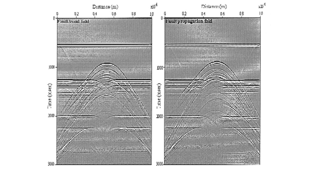
As in the Baysal example, the two unmigrated seismic responses show little resemblance to the actual models except where the layers are flat. The power of migration is its ability to move this surface- recorded energy back into its proper depth location. We will assume, for the moment, that we have perfect estimates of the velocity field. This is a big assumption since the problem of velocity estimation itself is a major problem (perhaps the major problem for prestack migration!). Zhu et al. (1998) have shown how we can use migration itself to estimate migration velocities.

The depth images in Figure 4 for the fault-bend fold and fault propagation fold examples show that migrations can unravel the unmigrated seismic sections and produce depth images that do clearly distinguish between the two models.

Conclusions

Seismic migration, one of the earliest applications of time reversed wave propagation, is routinely applied to millions of traces every day. Whether it is applied in two or three dimensions, in time or in depth, before or after stack, isotropically or anisotropically, acoustically or elastically, this workhorse technology has evolved from its earliest days as a mechanical, kinematic procedure to its modern incarnations based on the wave equation. This basis in the wave equation has provided inspiration for many ingenious researchers, including those who first recognized the potential applications of running the wave equation in reverse.

Clearly we are able to see the robustness of the reverse-time migration algorithm used in this study. The final migrated sections directly mimic the original models. All horizons seen in the original models in Figure 2 are imaged in the migrated sections seen in Figure 4. All hangingwall and footwall cut-offs are evident. The forelimb and backlimb are clearly imaged as are the set of parallel reflectors in the hangingwall and footwall.

Some migration artifacts are visible, primarily multiples. This is the likely result of not smoothing the velocity models prior to migration. Perhaps a more smooth velocity model would generate a result that has less migration artifacts, but overall the migrated sections are clear and concise.

It is impressive how the migration process is able to move reflection energy to its correct position in the subsurface. However if one views this in terms of time-reverse acoustics, perhaps the process is not mysterious. After all, if waves can be moved backward in time, we can move the seismic arrivals back to their reflection points. Time- reversed acoustics has found applications in many fields in addition to seismology. One wonders how many other applications await if we could turn back time in wave propagation.