Chasing Density – An Introduction to Seismic Acquisition, Processing, and Interpretation Methods Leading to Quantitative Interpretation

For any given reservoir or resource play, there are geological and geophysical measurements that impact the exploitation of in-situ hydrocarbons. Correct interpretation of these measurements is important to the overall economic success of an Exploration and Production company’s endeavors. As geoscientists, the integration of our conditioned geological and geophysical data in regards to reservoir engineering, drilling, and completions need to be done in a meaningful way. One of these ways is to use and analyze log responses from previously drilled wells.

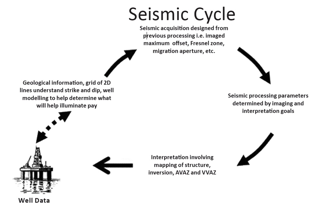
Various log curves help identify components of a reservoir such as the stratigraphy, structure, and rock properties inherent in the subsurface (Hunt et al, 2012). Well logs are important for geophysical work as we can cross-plot measured and/or derived properties that are achievable through seismic methods and manipulations. For instance, if a key play driver were porosity, an acoustic impedance and porosity well crossplot could direct one towards an acoustic impedance inversion if there was a reliable correlation. However, there is a large resolution difference between well logs and seismic data. Well logs can be up-scaled to seismic frequencies as well as synthetically modeled to overcome this resolution disparity. Understanding vertical resolution limitations of seismic data leads to the identification of which rock properties can be appropriately utilized (Hunt et al, 2012). This knowledge can influence future seismic survey design and the processing parameters chosen, so that the eventual interpretations are tailored for the target reservoir (figure 1).

A myriad of seismic attributes can be derived from the seismic data (figure 2) but all of these seismic attributes can be broken down into two categories:

1. Geometrical Attributes (Structural) – Attributes that enhance the visibility of the geometrical characteristics within seismic data. Examples include dip, azimuth, continuity, etc.
2. Physical Attributes (Stratigraphical) – Attributes that enhance the lithological properties inherit in seismic data. Examples include frequency, amplitude, phase, porosity, etc.

Most plays have both structural and stratigraphical elements that need to be understood properly to characterize a reservoir. The link between these types of seismic attributes to well, completion, and production data is crucial to this characterization. As mentioned previously, a stratigraphical attribute like acoustic impedance may indicate rock porosity that is known to be important for good production within a reservoir. As well, a structural attribute such as semblance can highlight lateral discontinuities important to finding features such as sand channels. The combination of these two example attributes can significantly hone exploration efforts if the main goal is to identify and drill porous sand channels.

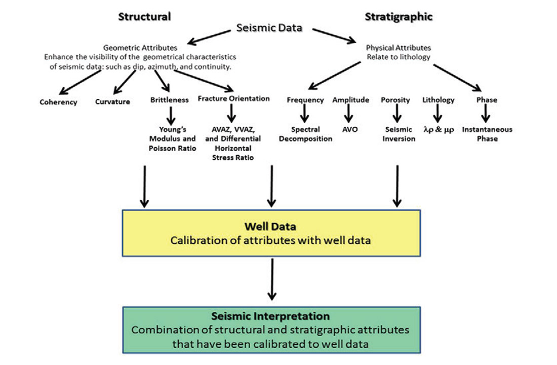
Within interpretation software packages today, there are simple ways to enhance features inherent in these structural and stratigraphic volumes. Once key attributes for a given reservoir are identified, the creation of uniformly spaced intervals between two interpreted seismic horizons (stratal slices) can aid overall seismic interpretation (Zeng, 2006). Another prospecting tool is the ability to blend attributes by colour and opacity. Simple colour blending combines up to three attributes by assigning each separately to red, green, and blue colours. Important geologic features can be made visually appealing and into a play risk or ‘fairway’ map by manipulating the attribute colour combinations.

All of these elements contribute to the understanding of the subsurface, and leads to making informed decisions in:

1. Purchasing leases in land sales
2. Whether or not to participate in a proposed partner drilling operation
3. Offset drilling requirements

These scenarios need to be considered by an asset team and sometimes require a swift response if there is little time to act. Having the pertinent information available for these occasions may avoid poor capital commitments.

Density

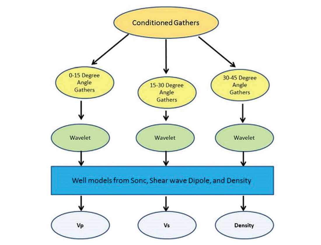
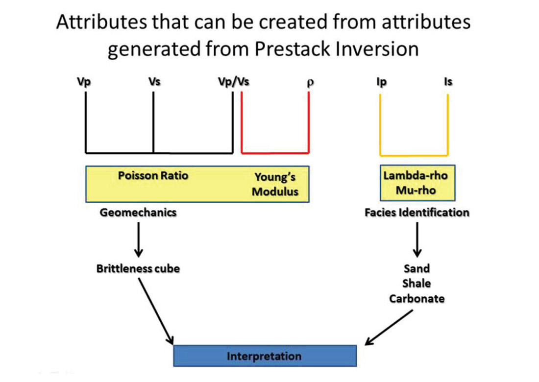
A volume of density is obtainable from conditioned pre-stack seismic data, along with p-wave and s-wave volumes, by means of a ‘joint’ or simultaneous pre-stack inversion (figure 3). Through the combination of these inversion products, other seismically derived rock properties such as Poisson’s Ratio, Young’s Modulus, Lambda-rho, and Mu-Rho can be calculated. Another key attribute obtained from these pre-stack inversion derivatives is brittleness. Brittleness has become widely used to help characterize unconventional plays and is calculated using Poisson’s Ratio and Young’s Modulus. However, density as a seismically derived attribute has been long viewed as unreliable for various reasons, those of which will be reviewed later.

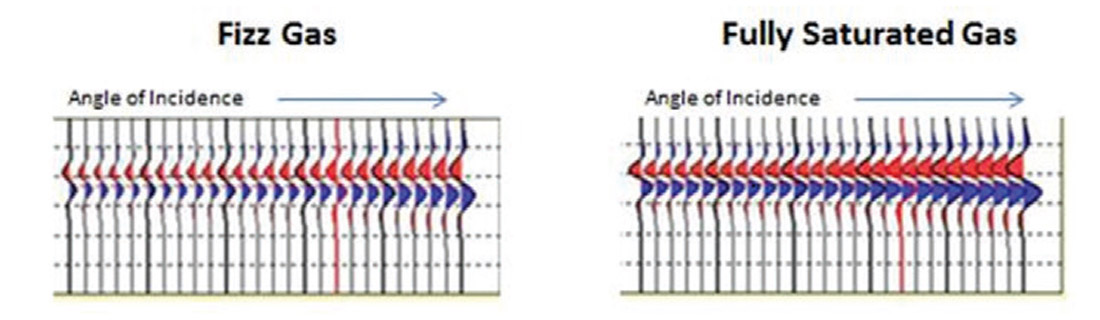
However, density can be utilized in many ways for successful reservoir characterization. An example of a density’s use relates to a characterization problem known as ‘fizz gas’ in certain reservoirs. Fizz gas is a term used to describe reservoirs that are very lowly saturated in gas (Sg < 10%). These reservoirs look like promising drilling prospects due to the fact that a just a small amount of gas will cause a large change in p-wave velocity, which coincidently has a similar seismic and amplitude versus offset (AVO) response to that of a highly gas saturated reservoir. There have been many failed exploration endeavors due to this problem. Density can be used to distinguish low and high gas saturated reservoirs as the bulk density response of a fizz gas reservoir is ten percent higher than that of a highly gas saturated reservoir (Han and Batzle, 2002).

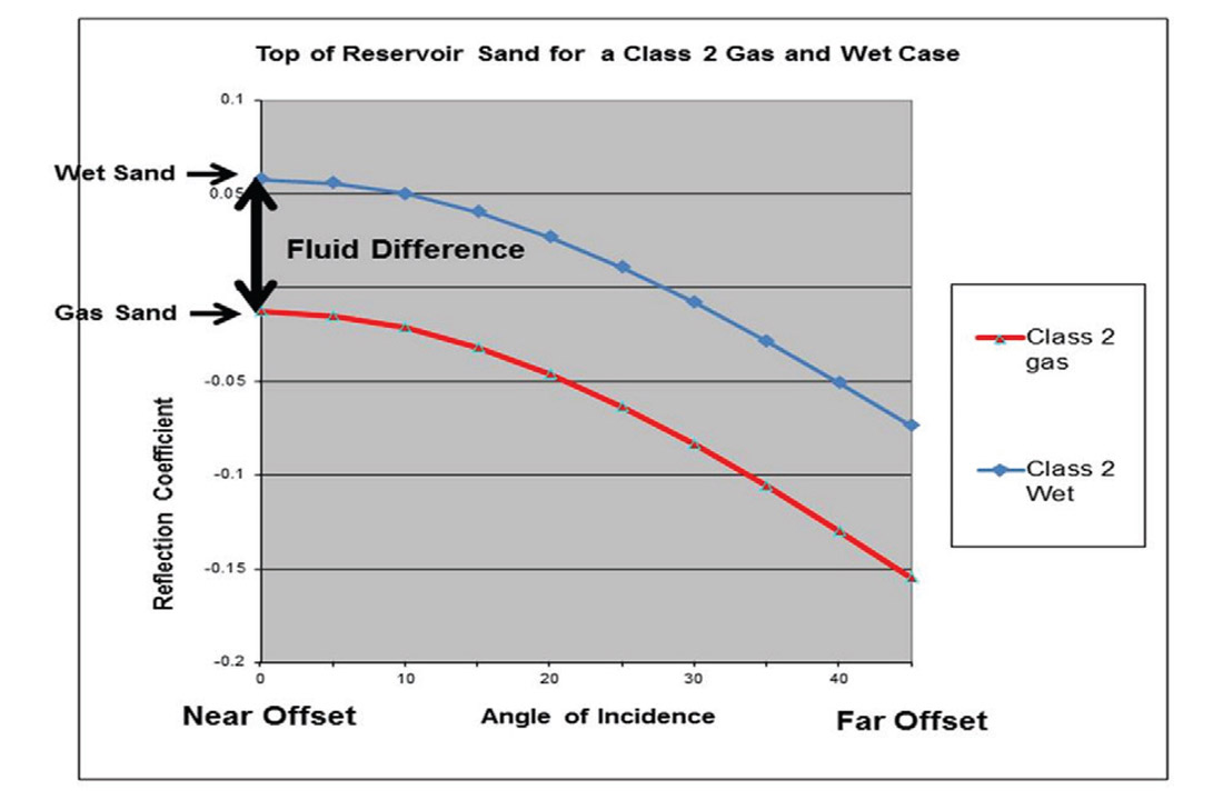
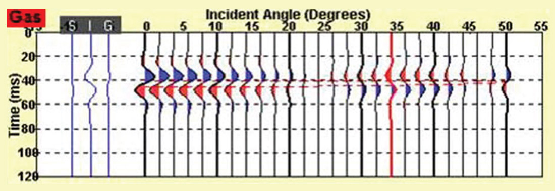
AVO anomalies caused by fizz gas reservoirs are hard to distinguish from gas saturated reservoirs (figure 4), but can be reliably verified through fault seal analysis. If a reservoir’s seal has been broken by a fault, the gas may slowly leak out into the overlying formations depleting the reservoir creating a fizz gas scenario. This type of analysis is rarely done prior to the unsuccessful exploration of a fizz gas reservoir. However, the viability of an AVO anomaly can be tested if it conforms or does not conform to the geologic structure in which it is occupying. If the anomaly conforms, a gas saturated reservoir is expected to be encountered.

Using Shuey’s (1985) definition of AVO response (figure 5), the density component of a gather can be isolated using the angle of incidence. Gathers are broken into three components based on the angle of incidence; a near-offset term from 0° to 15° that relates to the intercept, a mid-offset term from 15° to 30° that relates to the gradient, and a far-offset term from 30° to 45° that describes the curvature. If these terms are manipulated such that the intercept is subtracted from the curvature, an isolation of density is obtained.

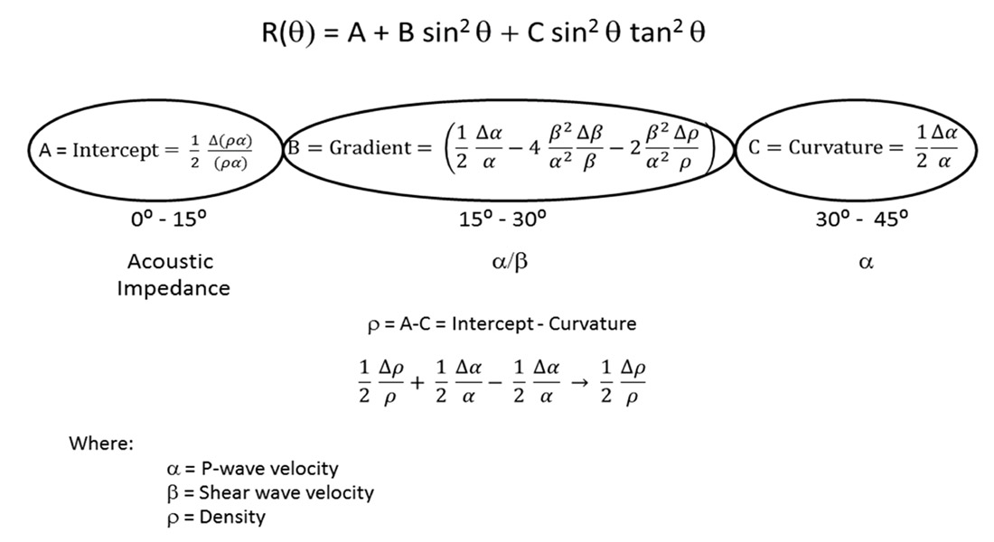
Since the curvature term is being derived from angles of incidence greater than 30°, there are significant limitations to its usefulness as issues in acquisition occur at these far-offsets that many seismic processing flows try to deal with. Problems such as move-out calculations and multiple elimination are mitigated in seismic processing. In order to trust the curvature term, a greater investment needs to be made during the acquisition stage to obtain better far-offset data (particularly in land surveys). Improvements made to survey design will benefit near-offset data as well, resulting in better inversion results and density approximation.

Seismic Acquisition

In order to acquire further far-offsets during seismic acquisition additional receivers need to be turned on or laid out, and both are fairly inexpensive to do when compared to the initial mobilization of the recording crew. A prior rule of thumb was that a receiver’s offset should be equal to that of the target’s depth, but in order to get proper angles of incidence to produce a reliable curvature term the ratio between offset and target depth should be 1.75. For example, if a target was known to be roughly 2000 meters deep, the furthest offset attempted for needs to be greater than 3500 meters.

In order to acquire better near-offset data, there is a need to reduce line spacing and add additional source points, but doing so raises the price of seismic acquisition significantly. There have been recent ideas proposed in seismic acquisition such as using a single vibrator, doing a single sweep at more locations, instead of traditionally having multiple vibrators at fewer locations. This method would acquire denser data, or further offsets, rather than a stronger signal at far fewer source points.

Additional seismic acquisition tools and methods such as nodal systems and simultaneous vibroseis acquisitions can lead to higher density surveys. Although 5D interpolation has become increasingly popular in recent years for seismic processing, it may have negative impacts on seismic acquisition efforts. Many acquisitions have been reduced in source and receiver density as 5D is able to infill traces at a significantly reduced cost compared to acquiring raw data. It is important to keep acquisition density as high as possible, since 5D will typically infill many more middle-offsets than near and far-offsets, which are crucial to interpretation.

Seismic Processing

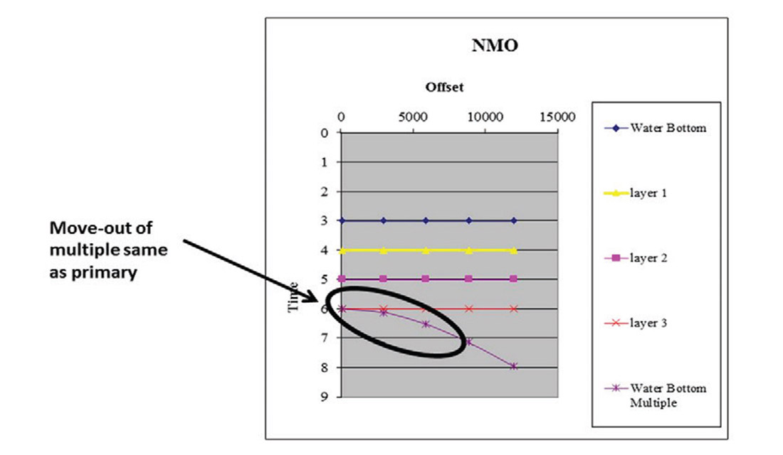
Having acquired seismic data, it is good idea to approach the processing or re-processing of a data set with an understanding of ideal deliverables, especially if reliable density volumes are required. Processing workflows can be highly tailored to suit these needs, especially if AVO compliance is necessary for good far-offsets and ultimately density. A major issue with near-offsets however is multiple contaminations. Multiples can disrupt near offsets (figure 6), since they have a similar move-out or ΔT to that of primary events; it is hard to remove them without affecting the actual signal. It is important that these multiples be removed as near-offsets help improve fluid knowledge in AVO classification and seismic attributes such as acoustic impedance.

Recent processing technology called Surface Related Multiple Elimination (SRME), developed by Delft University, can predict surface related multiples from the acquired data and does not require additional information. The strength of SRME is that it can adaptively account for mismatches of amplitude, phase, and source wavelets between multiples and primary reflectors (Verschuur and Berkhout, 1997; Dragoset et al, 2006; Lui and Dragoset, 2012). SRME is also capable of removing interbedded multiples, all while preserving the original signal.

Decontaminating seismic data of multiples allows for better, truer amplitudes on nearoffsets. It is then possible to achieve better seismic attributes such as acoustic impedance and with Acoustic Impedance we can gain information such as porosity and fluid content since the fluid information can be found on the near offsets (figure 7).

While SRME removes multiples from near-offsets, there is still a need to apply additional techniques to handle multiple effects on far-offsets. These can be handled by a noise reduction and multiple removal process known as Parabolic Radon Transform or a high resolution Radon proposed by Sacchi and Ulrych (1995). Radon transforms can eliminate multiples by fitting parabolas to recorded reflection events; multiples are parabolic in shape (in time-offset plots) compared to primaries, the process can then be instructed to remove events that appear to be multiples once it has fit a parabola to them. High resolution Radon eliminates multiples by separating events in Tau-p space (time versus slowness), and then applying a mute (figure 8).

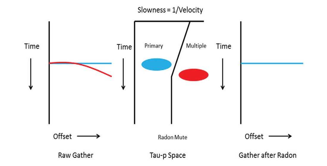
A mute can be designed within Tau-p space to eliminate multiple signals from the gather. High resolution Radon can typically separate multiple events better than normal Radon transforms as they usually do not overlap at all in Tau-p space, given a proper mute is applied. An improper mute will allow some energy from the multiple to return to the Time-Distance domain, causing the primary to be aliased (brightening of near-offsets). In deep water seismic, some run a Radon rather than an inside mute to remove this aliasing.

Other seismic processing advancements such as noise attenuation allow for better AVO compliant data. Noise has certain characteristics to it that can be modeled in different seismic domains, and then isolated within real data. Noise within the data can then be surgically removed enhancing the signal without harming it.

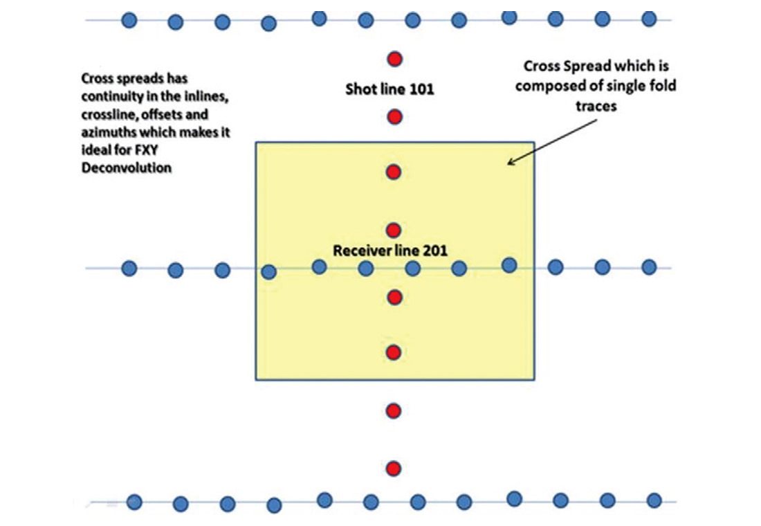
A recent targeted area for focused seismic processing is the crossspread domain (figure 9), where all geophones in a given unique receiver line are recording shots from a given unique shot line. The cross-spread domain is a continuous 3D subset of the 5D pre-stack wave field, which is comprised of inline, cross line, offset, absolute offset, and azimuth (Vermeer, 2007). It varies smoothly from trace to trace in each of the 5 spatial attributes.

There have also been recent developments in interpolation and regularization techniques, processing methods that fill in missing data for certain domains while regularizing the fold of the data. Missing data or irregular fold creates aliasing artifacts during pre-stack time and depth migration. This is because pre-stack migration relies on constructive and destructive interference to image the data. Regularized data is necessary to perform advanced interpretations such as seismic inversion, AVAZ, and AVO.

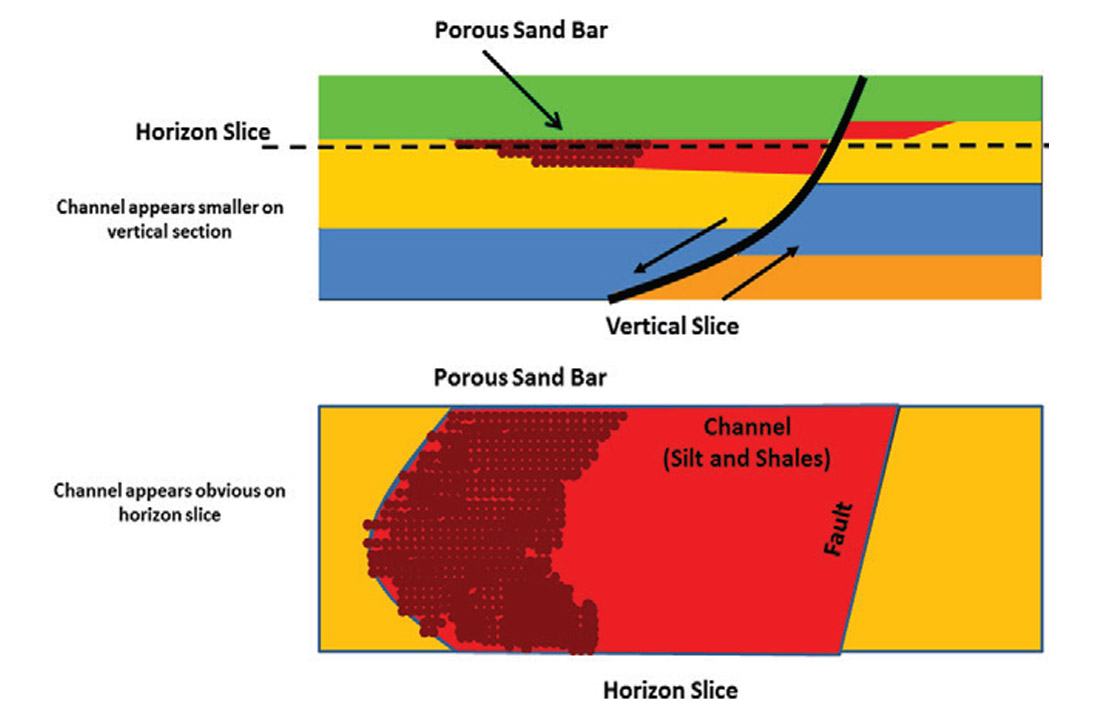
One such interpolation and regularization technique is 5D interpolation. 5D interpolation fills insufficient data areas in seismic surveys, especially in the near-surface, and is capable of reducing various noise sources. For example, 5D interpolation can decrease the effect of an acquisition ‘footprint’ that is easily seen in horizontal slices of seismic data. This is important for the imaging of some reservoir bodies, such as channels (figure 10), as they have great lateral extent rather than vertical (Zeng, 2006). Improving the fidelity in time, horizon, and stratal slices directly benefits the ability to reliably map these sometimes small geologic bodies.

NMO and Imaging Higher Incidence Angle Data

Processing seismic data beyond 30° (incidence angle) becomes critical in the chase for a reliable density. Many processing algorithms are designed for an incidence angle of 30° due to the prior rule of thumb mentioned, where offset is equal to depth. Such is the case for the standard two-term normal move-out (NMO) equation as well as imaging methods like straight ray pre-stack time migration.

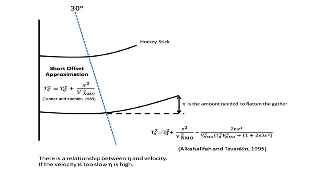
The two-term NMO equation however fails beyond 30° (incidence angle) and causes a rather dramatic effect called ‘hockey sticking’, where an event (peak or trough) turns upwards in the far-offsets of a gather, appearing similar to the shape of a hockey stick (figure 11). This problem, more detailed, is due to the fact that NMO is plagued by a short offset approximation associated with Snell’s Law; as velocities change between different geologic layers, curved ray paths occur instead of straight ones. Velocities then change with offset, creating the hockey stick effect. NMO ‘stretch’ is another common occurrence, where there is a shift toward lower frequencies in the far-offsets. The combined result of this stretching of frequencies and hockey sticking causes the wavelet to be significantly altered. An assumption made by Shuey’s (1985) approximation is that the wavelet used is supposed to be constant, so there is a need to deal with these NMO problems if AVO characterization is required (Cambois, 2002).

The short offset approximation for the two-term NMO equation is:

The non-hyperbolic move-out is generally handled by a third and fourth order NMO equation such as:

NMO stretch can be mitigated when using at least an extra term since it defines the shape of the parabola better in move-out. Generally, η is used to flatten the hockey stick effect in far-offsets.

η can be thought of as a ‘fudge’ factor to obtain flatter gathers. η is one of the Thomsen parameters and can be related to ε and δ through the equation η=(ε-δ)/(1+2δ) (Thomsen, 1986).

Straight ray pre-stack time migration (PSTM) produces the same issues since ray paths in real data are curved. Migrating data with a Kirchhoff straight ray PSTM will result in hockey sticking due to curved data, but also to vertical transverse isotropy (VTI). VTI can occur in geologic formations as the same properties may occur laterally within rocks, but may also vary throughout the vertical extent of them. A lithological example of such a rock is shales. Although VTI’s effect on data is expected to be weak, data corrected for curved ray paths exhibits hockey sticking, suggesting that VTI is large enough to require additional processing. These problems have resulted in the shift in processing flows to curved ray PSTM instead of straight ray methods.

Curved ray PSTM take into account bent ray paths that occur in a velocity changing medium. It can be run in several ways:

1. Through ray tracing
2. Using a fourth order move-out equation, where η is reasonable to 18000 feet
3. Using a sixth order move-out equation

Solving for curved rays has the additional benefit of imaging anisotropy through VTI as well as η being representative of certain rock properties. Prior to curved ray PSTM, the difference between time and depth migration was how each treated curved rays, with depth migration being able to account for them. However, the difference now is that time migration utilizes stacking velocities to flatten gathers. Time migration inverts stacking velocities to interval velocities, producing physically impossible values. It is obvious then that the result of time migration is to simply produce and image, which is not necessarily geological valid.

In depth migration, interval velocities will have representative values of the geologic units. Depth migration’s velocity field is created using seismic horizons, sonic log responses, check shot data, and vertical seismic profiles (VSP’s) in an attempt to accurately model the Earth’s subsurface. Seismic wave behavior is then modeled better through depth migration than time migration (Gray et al, 2001). Whenever there is a known rapidly-varying lateral velocity, pre-stack depth migration is the correct process to use. However, time migration still has its own advantages over depth migration. Time migration is computationally inexpensive, is less sensitive to velocity, and adequately images most reservoirs for interpretation purposes. If pre-stack depth migration is chosen, there needs to be an appropriate geological model built while time migration can be run for initial results.

Another problem with wide azimuth data is horizontal transverse isotropy (HTI), similar to VTI, which produces a sinusoid shape to the gathers. HTI parameters, as well as VTI, are being used in proprietary pre-stack time migration algorithms; producing more accurately positioned dipping and faulted planes. These methods preserve correct offset amplitude information, especially in far-offsets (McLain, 2013).

AVO attributes are calculated through a linear regression of a single sample’s amplitudes. If gathers are not flat, AVO attributes will have an inherit noise within them. Amplitude leakage from the intercept into the gradient is a common problem (Hermann and Cambois, 2001; Cambois, 2002). AVO attributes such as the ‘fluid factor’ may be reduced to the far-offset stack (Cambois, 2002), it will also cause the gradient to be an order of magnitude noisier than the intercept (Whitcombe et al, 2004). Again, gathers need to be properly flattened to compensate for these affects. Some processing methods such as trim statics attempt to fix the litany of problems caused by residual and higher order move-out, vertical transverse isotropy (VTI) and horizontal transverse isotropy (HTI). There is difficulty and risk in trim statics, where some AVO anomalies like class 1 (figure 12) and 2P cases can be miss-aligned destroying their AVO response.

In these types of AVO anomalies, it is apparent that aligning for a maximum energy there will be issues picking the correct velocities. In order to obtain optimal velocities for these classes, methods such as Automatic Continuous High Density High Resolution (ACHDHR) velocities like Swan’s velocities may be used. These velocities use a Residual Velocity Indicator (RVI), which is a real part of the intercept convolved with the gradient’s conjugate (Swan, 2001). Using RVI, velocity errors within the gradient are reduced, resulting in flatter gathers and better AVO attributes.

Seismic Inversion

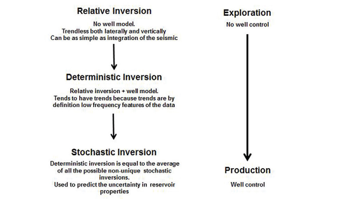
Although many seismic surveys have data that is beyond a 45° angle of incidence, the data has to be correctly processed to have reliable near-offsets, far-offsets, and therefore seismic inversion. Different types of inversions will produce different solutions as there many combinations of p-wave, s-wave, and density values in the original seismic signal. This problem of non-uniqueness can be addressed through the comparison of different inversion results (figure 13), such as the following:

1. Relative Acoustic Impedance – This type of inversion is directly estimated from the seismic data, with no other inputs. It is fairly robust and is generally used in exploration scenarios where there is limited or no well control. Relative inversions are trendless vertically and laterally due to the lack of low frequency features inherit in the seismic data.
2. Stochastic Inversion – Stochastic inversion uses multiple solutions and statistically verifies them against production data and key measurements to calculate rock parameters.
3. Deterministic Inversion – This inversion is constrained by the solutions of well models. Low frequencies are replaced by these well models in the inversion process. Deterministic inversions are averages of all possible non-unique stochastic inversions.

Results from these inversion types can be used to estimate reservoir properties’ uncertainties. These uncertainties arise from a stochastic inversion’s statistical calculations. Uncertainty in lithology, porosity, and overall reservoir connectivity can be produced in the form of probability maps and volumetric measurements.

Attempting more than one type of inversion helps verify the validity of the rock properties produced. Having multiple forms of the properties allows for the use of a geostatistical neural net; an algorithm that predicts seismic attributes based on the correlation of reservoir properties to a targeted attribute. Ultimately, the goal of these predictive software solutions is to create numerous quantitative rock properties to aid seismic interpretation (figure 14), known as Quantitative Interpretation (QI). QI is the tying of multiple seismic data, various attributes, and conditioned geological or engineering data in a way that adds considerable value to the characterization of a reservoir. To perform QI, a set of reasonable questions should be in mind in order to identify the rock properties pertinent to a given reservoir (Hunt et al, 2012).

If these attributes successfully correlate to initial well log observations, an extrapolation to further attributes can be made. Neural nets allow for multiple inputs and iterations, substantiating derived rock properties such as density.

Conclusion

nitially, seismic should be acquired to have an appropriate amount of data at 0°-45° angle of incidence for a zone of interest. Next, processing methods need to maintain the truest primary signal for this set of data. Finally, inverting this seismic data multiple ways helps resolve the non-unique problem. Once multiple sets of rock properties and attributes are produced, neural nets can find specific combinations of these inputs to recreate targeted properties.

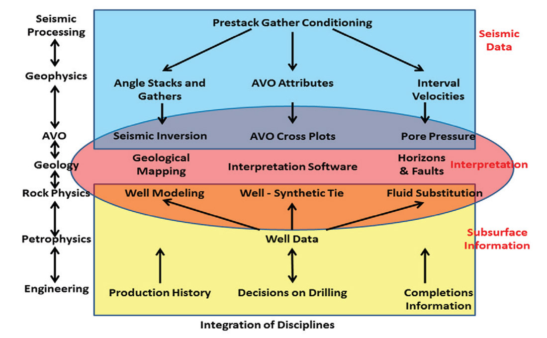
The aforementioned work not only identifies drilling locations, but can shape ongoing drilling and completions efforts, benefitting exploration and development. Reservoir models are improved integrating the geological, geophysical, and engineering disciplines.

Key elements such as completion and production information tend to not be included in geological and geophysical analysis. These efforts should be regularly fed back into interpretations to have an up-to-date model at all times (figure 15). Quantitative interpretation can become static, leading to potentially poor reservoir characterizations when moving to new drilling locations.

This type of work is routinely done in offshore environments due to the high costs of drilling wells. In a mature oil and gas area like the Western Canadian Sedimentary Basin, the cost of drilling and completing a well is relatively inexpensive. There is not necessarily a need to do the level of interpretation discussed in this paper. Seismic is sometimes dismissed as the amount of well control in Alberta is immense. However, this information can bolster seismic interpretations in such a way that should not be ignored. Through a similar workflow described in this introduction, seismic can be taken to another level, expanding a company’s economic possibilities through quantitative interpretation.

Acknowledgements

The authors would like to acknowledge Laurie Bellman of Canadian Discovery and Bill McLain of Global Geophysical for their input. Some of the ideas and concepts expressed in this paper came from discussions with them. Without the numerous challenging questions of our junior geologists and geophysicists at Talisman, such as Ryan Cox, this article would not have come to be. A special thank you to all those who helped edit this article as well. Finally, the authors would like to thank Talisman Energy for allowing us to write this article, specifically Rick Warters and David D’Amico.