Case study: 3C and 9C prestack shear wave splitting analysis at Big Sky

We present a tutorial style case study in which we compare two approaches to shear wave splitting (SWS) analysis and layer stripping on a subset of 3-D 9-C data from Montana. The first, and perhaps more familiar method, utilizes converted wave, or PS data, while the second utilizes pure shear wave data. We also incorporate results from PP processing in the study. The objective is to compare essentially direct measurements derived separately from pure P and S mode datasets to the indirect mixed mode measurements derived from PS data processing. SWS attributes derived from 2C X 2C data compare favourably to the corresponding PS results. The PP stacks and layer stripped SH stacks have comparable structural features. We investigate the relationships between time delays estimated from PS data, SV, and SH data. As expected from theory, traveltime delays between fast and slow modes estimated from pure shear wave data are about twice as large as the time delays estimated from converted wave data. However, time delays estimated from SV data are slightly higher on average than those estimated from SH data. We also investigate the relationships between fast azimuths estimated from PS, SV, and SH data. Again as expected from theory, we show that SV and PS SWS analyses predict similar azimuths, and that estimated SV and SH fast azimuths tend to be orthogonal to each other. We also show that this agreement with theory improves beyond a threshold magnitude of SWS, simply because azimuth estimation becomes unstable for negligible amounts of SWS. Specifically, agreement with theory is good when PS splitting estimates are greater than about 2ms and SV splitting estimates are beyond 4ms.

Background

SV and SH wave modes. SV and P modes are coupled, in the sense that each generates the other upon reflection or transmission at an interface, or discontinuity in the elastic parameters of the propagation medium. Both modes are characterized as having particle motion polarized in the vertical-radial (source-receiver) plane. P-waves are polarized in the propagation direction while SV waves are polarized orthogonal to the propagation direction. This statement holds for horizontal interfaces within isotropic, homogeneous media; more generally, the ‘vertical’ plane of propagation becomes the plane normal to the interface.

The SH mode is not coupled to other modes – it is polarized in the horizontal plane, perpendicular to both SV and P. Although SH and SV modes are generally subject to the same losses due to attenuation, conservation of energy together with the fact that SH waves are decoupled from P waves at least in part explains why SH events typically appear with stronger SNR than SV events. SV and SH waves also have very distinct AVO responses – SH tends to vary slowly with offset/angle while SV typically has a polarity reversal in the 20-25 degree range. Therefore stacking mutes tend to be more open for SH than for SV data, which means stacking fold, and therefore SNR, is higher for SH than for SV. We have repeatedly observed this AVO behaviour and corresponding SNR improvement after having processed many 9C datasets (see also Simmons and Backus, 2001).

Azimuthal anisotropy and shear wave splitting. The phenomenon of SWS is perhaps most readily understood in terms of a familiar form of azimuthal anisotropy: that induced by aligned vertical fractures or cracks in brittle, otherwise isotropic rocks (Martin and Davis, 1987). This is an example of HTI anisotropy, where HTI stands for ‘transverse isotropy with a horizontal symmetry axis’. ‘Transverse isotropy’ means the plane perpendicular to the symmetry axis is isotropic. The symmetry axis is perpendicular to the dominant fracture strike and dip. Both SV and SH shear modes undergo SWS when they encounter anisotropic, or birefringent media. In the case of HTI, both shear modes split into two orthogonally polarized shear waves, each travelling with potentially different velocities. When the HTI symmetry is due to vertical fracturing, the fast direction for SV waves (SV1) corresponds to propagation parallel to the fracture strike. For SH waves the fast azimuth direction (SH1) is orthogonal to the fracture strike. The corresponding slow directions (SV2, SH2) are orthogonal to the fast directions. More generally, the fast directions SV1 and SH1 are along and perpendicular to the symmetry axis, respectively – what’s fast for SV is slow for SH and vice versa.

We stress that any form of azimuthal (velocity) anisotropy causes SWS, and also that the cause need not be due to fractures. In fact, any small scale structure (sub seismic wavelength) within the medium exhibiting dominant directionality will suffice. For example, near surface clay tills contain clay particles which tend to be preferentially aligned, thereby manifesting as HTI anisotropy. Indeed, “tectonic and geomorphological processes such as crustal movements, tilting, moving ice sheets, erosion and solifluction may produce soils with stresses varying in different horizontal directions” (Graham and Houlsby, 1983). Indeed, we often see strong SWS in the overburden, and specifically in so-called non-compliant rocks (Cary et al., 2010) which tend not to support fracturing.

Influences on anisotropy strength may include elevated pore pressure due to injection, temperature increase over time, induced fracturing in brittle rocks, propping of fractures (e.g., Grossman et al., 2013), and the degree to which fractures are aligned.

9C acquisition. Notation: H1 = inline direction, H2 = crossline direction, V = vertical direction.

Data acquisition with two orthogonally polarized horizontal source components into two orthogonally polarized horizontal receiver components yields a 4C, or 2C X 2C dataset. The latter terminology, 2CX2C, is preferred in order to avoid confusion with the usual 4C case, where a 3C geophone and a hydrophone are used for simultaneous recordings. We label the components of the data in the field coordinate system as: H1H1, H1H2, H2H1, H2H2, where the first component, Hi, refers to the source polarization and the second, Hj, denotes the receiver component orientation (i ,j = 1,2). Including the vertical component, V, for both source and receiver, results in a 3C X 3C, or 9C dataset.

These are idealized field coordinates – in practice source-side data rotation is required to simulate a consistently oriented experiment, into true H1 and H2 components. Similarly, receiver orientations also normally need to be adjusted (see Grossman and Couzens, 2012 for an example of an automated method). This is due to reality constraints in the acquisition: typically, the vibe vehicle changes direction by 180 degrees each time it begins acquiring along a new line. Since the baseplate is either in line with the vibe or rotated in a direction perpendicular to it, the ‘first motion’ of the baseplate changes direction and the in-situ H1 and H2 source polarizations will alternate sign accordingly. Moreover, deviations from the nominal (expected) H1 and H2 directions frequently occur due to slight, and sometimes large, source and receiver misalignments. Fortunately these days, data supplied by the contractor include accurate vibe vehicle orientations at each source point, from which the source polarization directions can be deduced and subsequently adjusted. Mathematical details of these component rotations can be found, e.g., in Alford (1986), Thomsen et al. (1999) and Hardage et al. (2011).

Rotation from field coordinates to radial and transverse coordinates. In preparation for processing and SWS analysis, the sources and receivers are mathematically rotated into radial and transverse coordinates (Gaiser, 1999, Simmons, 2001), where the radial direction, R, is defined as the azimuth of the vector originating from the source and pointing toward the receiver, and the transverse direction, T, is perpendicular to the radial direction (Figure 1).

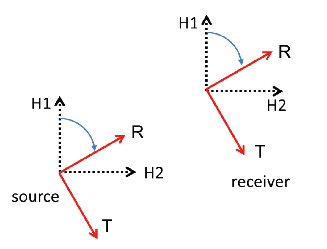
Just as is the case for converted wave data, this is the natural coordinate system for processing 2CX2C data (whether this processing coordinate system is ‘natural’ is not universally agreed upon!). Indeed, for isotropic, layered media, this coordinate system yields an orthogonal decomposition of the wavefield into SV and SH modes – RR and TT respectively; in theory, no coherent energy should appear on the cross-components RT and TR. As we will see, coherent energy on the cross components may be indicative of SWS.

Big Sky example: Indications of shear wave splitting

Limited azimuth stacks, or LAS’s, are azimuthally sectored stacks, sorted by source-receiver azimuth. When there is splitting, these stacks reveal azimuthal variations on events on all components: for 2C X 2C data, RR and TT events will show sinusoidal variation in traveltime with azimuth. Also, energy will have leaked onto the cross terms, RT and TR, and events on those LAS’s will show polarity reversals along the fast and slow directions. Similar properties apply for PS data, where LAS’s will show sinusoidal variations on the R component and polarity reversals along the fast and slow directions on the T component.

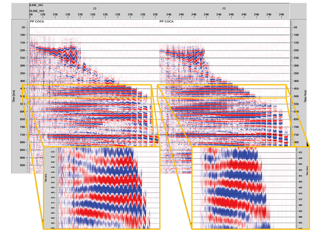
Figure 2 gives a preview of some graphical data representations used for diagnosing azimuthal anisotropy: from P wave data using a COCA volume (depicted in the leftmost panel – COCA volumes will be explained below); from PS data using a LAS (middle panel); and from 2C X 2C data also using a LAS (rightmost panel). The LAS’s have been rescaled vertically using a Vp/Vs ratio of two to yield a coarse registration of events. Overburden SWS analysis was conducted on 3C and 2CX2C data within the illustrated time window. Azimuths span 0 to 360 degrees in the LAS’s and 0 to 180 degrees in the COCA display.

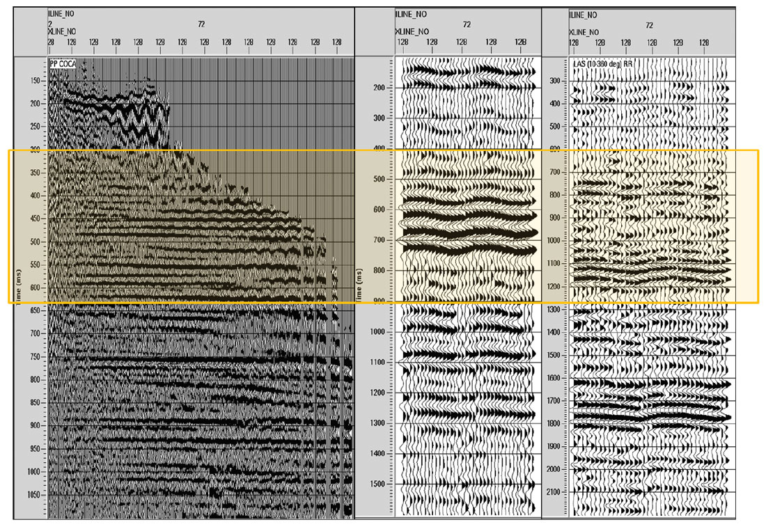
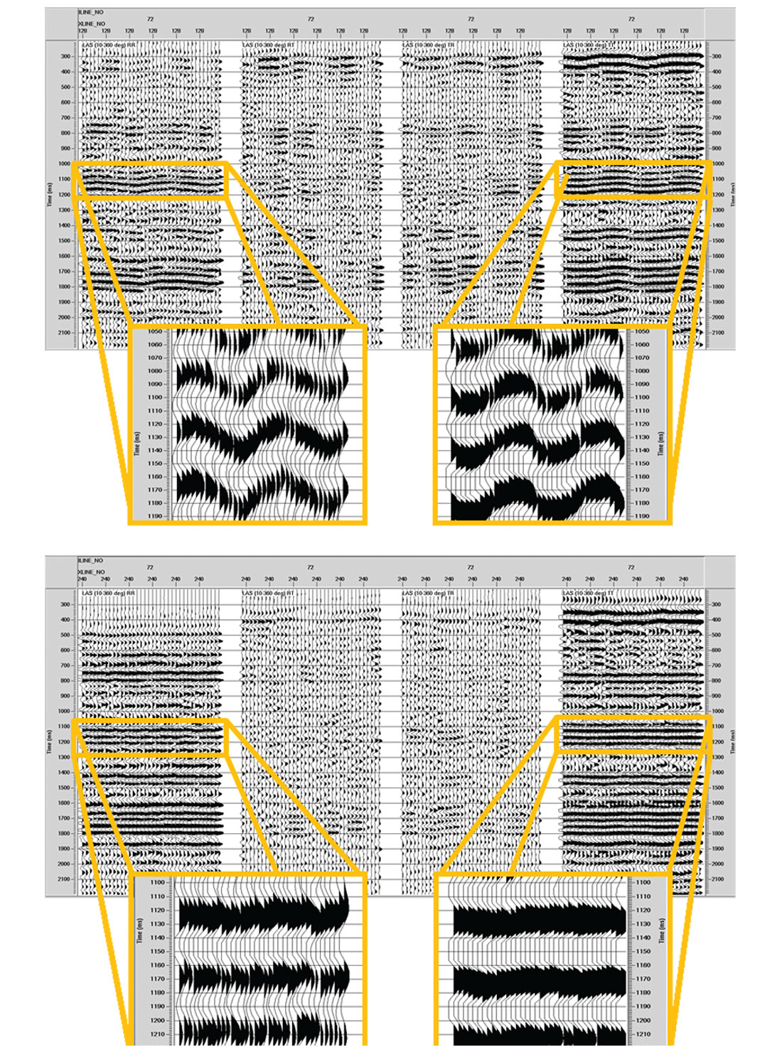
Figure 3 displays LAS’s for 2C X 2C data at location A (IL 72 and XL 128 – top display) and location B (IL 72 and XL 240 – bottom display). There is clear SWS signature at location A. Both RR and TT components show sinusoidal variation in traveltime with azimuth, while the cross components show events changing polarity (four times) with azimuth. Visual inspection of the magnified RR and TT events suggests traveltime delays of 20ms and 16ms, respectively between minimum and maximum arrival times on a given event. Location B shows very little indication of SWS. RR and TT events are quite flat and cross term energy is sporadic. Notice that the sinusoidal variations for RR and TT components are about 90 degrees out of phase with each other, i.e., peaks on one correspond to troughs on the other and vice versa. This is consistent with our observation that ‘what is fast for SV is slow for SH’.

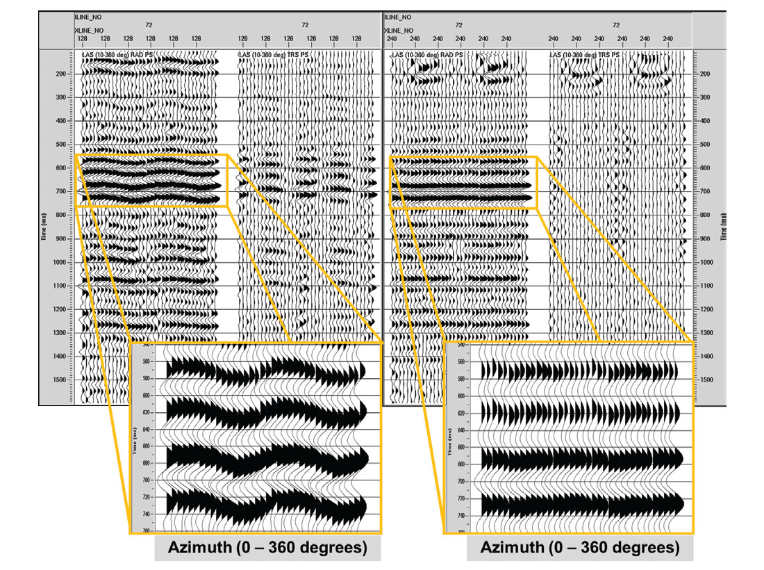
Similarly, Figure 4 displays LAS’s for PS data at locations A and B. Again, there is clear SWS signature at location A and very little at B. At location A, the R component shows sinusoidal variation in traveltime with azimuth, while events on the T component change polarity every 90 degrees of azimuth. At location B, R events are quite flat and cross term energy is incoherent. Visual inspection of the magnified R events suggests traveltime delays of 11ms and 2ms between minimum and maximum arrival times at locations A and B, respectively.

PP common-offset, common-azimuth (COCA) volumes. PP COCA volumes are created by binning P-wave traces into common source-receiver offset and azimuth ranges and then stacking within each of the resulting bins to assign a single trace per offset-azimuth bin (Gray, 2007). Traces from the COCA volume may then be sorted by offset, with azimuth as secondary sort key to enable visualization of azimuthal anisotropy.

Azimuthal anisotropy for P waves manifests as a sinusoidal variation in traveltime with source-receiver azimuth. This variation is negligible at zero offset and increases with offset as the raypaths become more horizontal and therefore more sensitive to the azimuthal velocity variation. The COCA volume displayed in Figure 5 clearly displays these traveltime characteristics of azimuthal anisotropy.

Big Sky example: SWS analysis and layer stripping

PS Layer Stripping. When R and T coordinates of converted wave data are aligned with either PS1 or PS2 directions, no splitting should occur, and no coherent energy should be present on the T component. Otherwise splitting occurs and energy leaks onto T. Using rotation operators, we can mathematically simulate an experiment in which H1 and H2 happen to align with the PS1 and PS2 directions. This process decomposes the PS wavefield into fast and slow SV modes. Therefore, to layer strip, we rotate to PS1, PS2 coordinates, shift events up on PS2 to align with the corresponding events on PS1, and then rotate back to the R, T system. This removes the effect of splitting, transfers coherent energy from T to R, and effectively replaces that layer with an isotropic one.

SWS analysis. Since the PS1 direction is not known a priori, we first perform a brute force scan over all possible azimuths and time delays and use some objective function to determine the solution – e.g. maximize stack power on the radial component (Li and Grossman, 2012), and then perform the layer stripping procedure as described above. This scanning procedure is referred to as SWS analysis.

2C X 2C Layer Stripping. The 2C X 2C case is very similar to the PS case, but is somewhat more complicated. It turns out that the time delays between fast and slow events for 2C X 2C data are twice those of corresponding events for PS data. This is because of the two-way traveltime delay in the pure shear wave case vs. a one-way, up-going delay after conversion in the PS case (Thomsen et al., 1999).

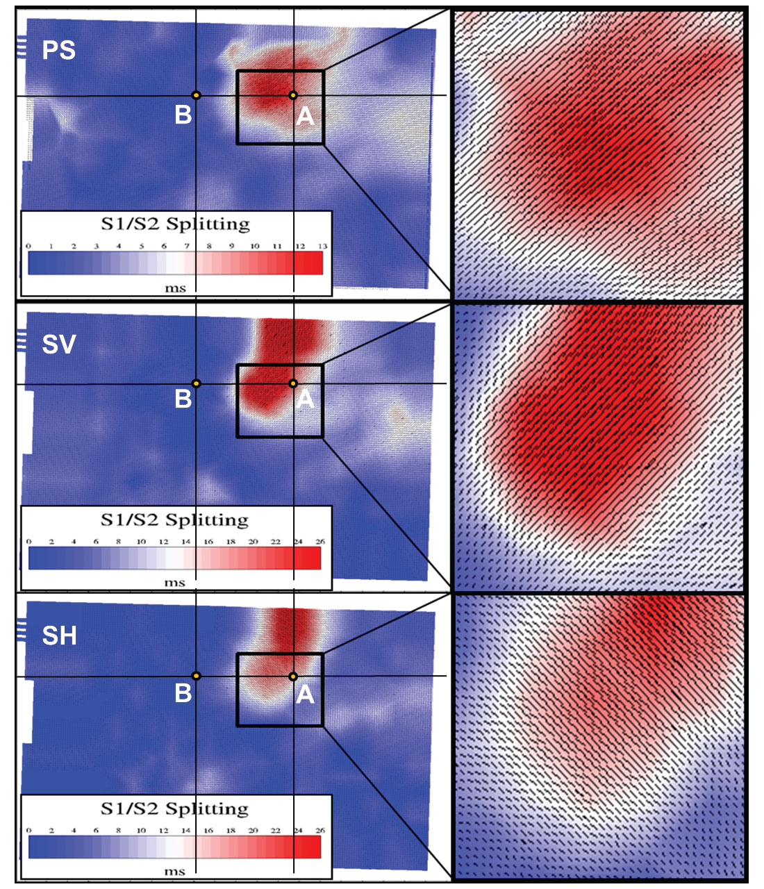
Figure 6 shows three SWS attribute maps derived independently from PS data, RR/ RT data, and TT/TR data. The SWS analysis was conducted to estimate overburden SWS using the data windows shown in Figure 2. Since SV and SH polarizations are orthogonal to each other, and because the polarization orientation dictates the speed of the wave, we expect SV1 and SH1 to be orthogonal to each other. This is indeed the case here. Also notice that the estimated time delays for the 2C X 2C case are twice those for the PS case, as expected. The actual time delay values used for the layer stripping at location A are as follows: PS1-PS2 delay = 11.2ms, SV1-SV2 delay = 20.4ms, SH1-SH2 delay =16.0ms. These compare very well to the values estimated by inspection of the LAS’s in Figures 3 and 4 (respectively, 12ms, 20ms, and 16ms).

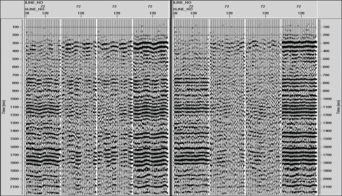
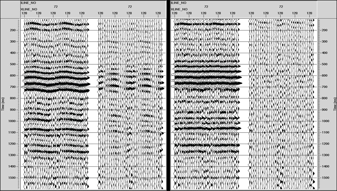
Figure 7 illustrates RR/RT/TR/TT LAS stacks at location A before and after layer stripping. Events displaying sinusoidal traveltimes with azimuth on RR and TT LAS’s are flattened after layer stripping, while cross term energy is greatly reduced. Similar results apply to the analysis and layer stripping of the PS data at the same location (Figure 8).

Discussion

Up to this point we have investigated only two locations within the survey. By inspecting the COCA volume for PP data and LAS’s for the PS and pure shear data, we consistently found little indication of azimuthal anisotropy at location B, and found clear indications at location A. The time delays estimated visually at A were 4ms, 12ms, 20ms, and 16ms, respectively, for PP, PS, SV, and SH data. Simply because of velocity differences amongst the wave modes, we expect time delay estimates to increase according to that observed order: PP, PS, and SS. For a more general picture, Figure 9 compares full azimuth PP stacks with TT stacks before and after overburden layer stripping along IL 72, which includes locations A and B (see Figure 6 for map view). As in Figure 2, the TT stacks have been compressed vertically for easier comparison to the PP stacks. Dim spots on the TT stacks are essentially healed by layer stripping, and structural details are comparable to the PP results.

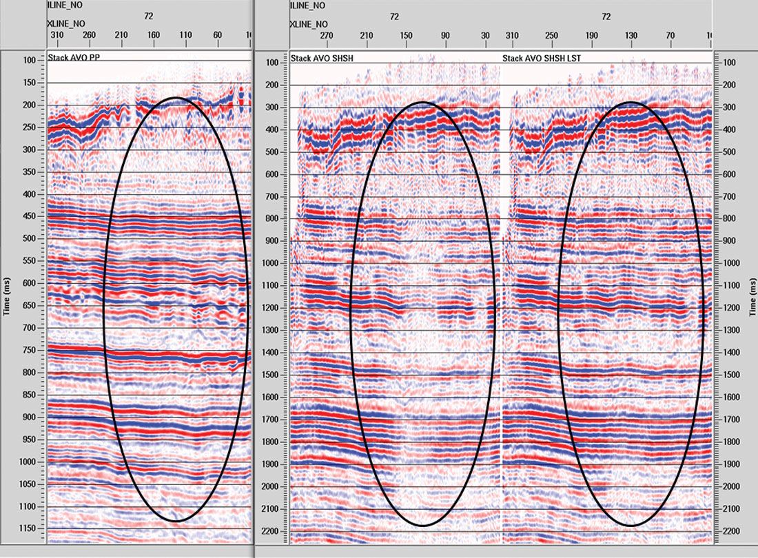
Figure 10 shows three crossplots illustrating the pairwise statistical relationships between fast-slow shear wave time delays estimated from PS, SV, and SH data. The yellow lines included in each plot define the theoretically expected relationships between the two variables being crossplotted. As expected, traveltime delays between fast and slow modes estimated from pure shear wave data are about twice as large as the time delays estimated from converted wave data. PS and SV estimated time delays have the best agreement. Time delays estimated from SV data are slightly higher on average than those estimated from SH data.

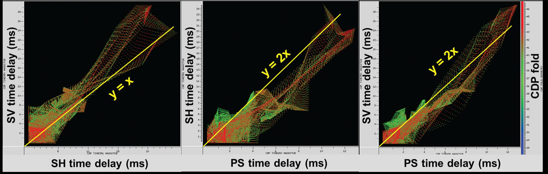
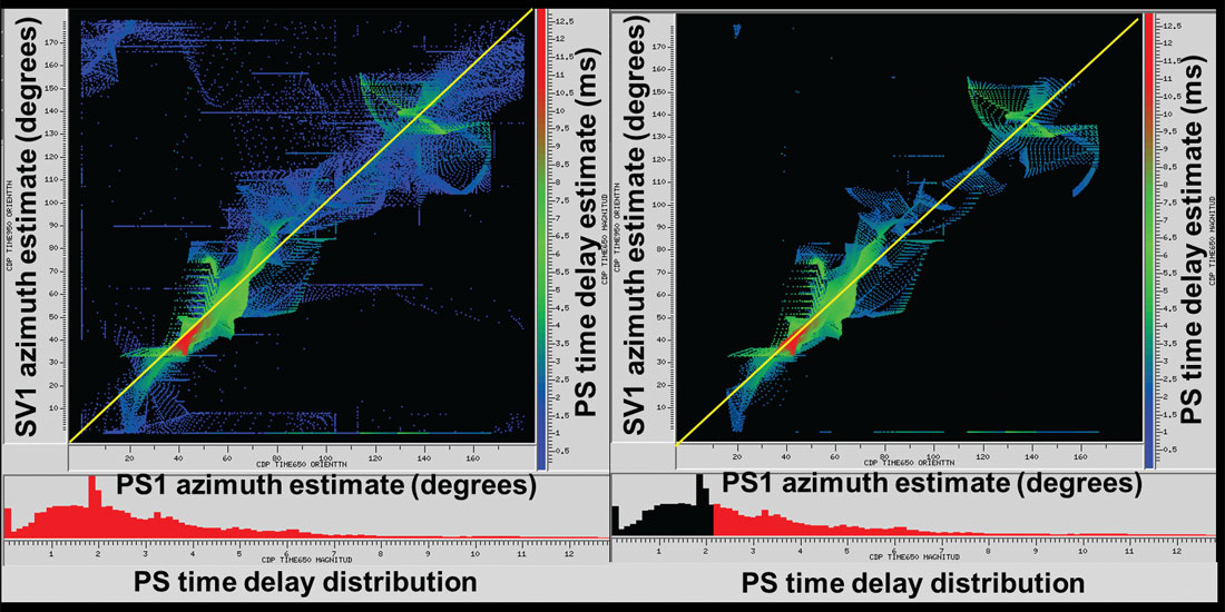
Figure 11 shows crossplots of fast shear wave azimuths, PS1 and SV1, respectively estimated from PS data and SV data. The plots are histogrammed and color coded by the PS-estimated time delays. The first plot includes all PS time delays, while the second excludes all time delays below 2.1ms. The yellow line indicates the line of equal azimuth estimates, which is theoretically expected. As can be observed by comparing the two plots, agreement with theory is good when PS splitting is greater than about 2ms. This is most likely due to the fact that azimuth estimation becomes unstable as SWS delays become negligible (Li and Grossman, 2012).

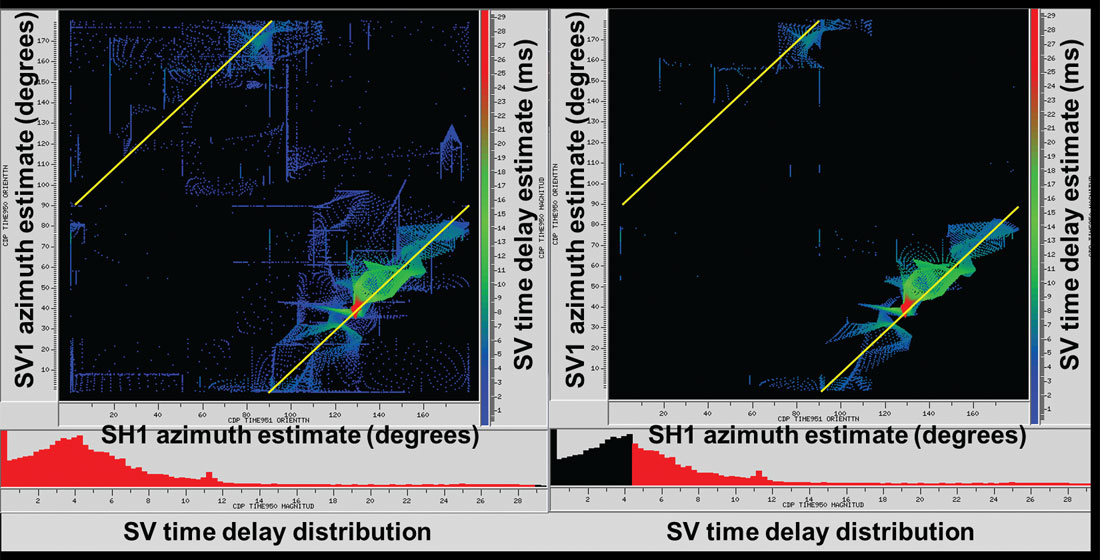
Similarly, Figure 12 shows crossplots of fast shear wave azimuths, SV1 and SH1, respectively estimated from SV data and SH data. The plots are histogrammed and color coded this time by the SV-estimated time delays. The first plot includes all SV time delays, while the second excludes all time delays below 4.2ms (twice the 2.1ms threshold for PS time delays used in Figure 11). The yellow line indicates the theoretically expected relationship of azimuth estimates – a 90 degree difference (modulo 180 degrees). Again as can be observed by comparing the two plots, agreement with theory is good when SV splitting is greater than about 4ms.

Conclusions

We discussed some background theory and practicalities concerning SV and SH shear wave modes, azimuthal anisotropy and SWS, 9C acquisition, rotation from field coordinates to radial and transverse coordinates, indications of SWS, layer stripping, and SWS analysis. We investigated two approaches to SWS analysis and layer stripping, separately utilizing converted wave and pure shear wave data. We also incorporated results from PP processing in the study. We compared direct measurements derived separately from pure P and S mode datasets to the indirect mixed mode measurements derived from PS data processing. We found that the SWS attributes derived from 2C X 2C data compare favourably to the corresponding PS results, and that the PP stacks and layer stripped SH stacks have comparable structural features. We investigated the correlations between time delays estimated from PS, SV, and SH data. It was found that SV SWS analysis predicted slightly higher time delays on average than SH SWS analysis. As expected, time delays estimated from SV SWS analysis correlated well with those from PS SWS analysis, with SV delays averaging about twice the PS delays. Similarly, time delays estimated from SH SWS analysis correlated well with those from PS SWS analysis, with SH delays averaging slightly less than twice the PS delays. Generally, time delays due to azimuthal anisotropy between fast and slow azimuths for PP events were found to be smaller than those for PS events, and these delays in turn were smaller than those for pure shear events. We also investigated the correlations between fast azimuths estimated from PS, SV, and SH data. As expected, it was found that SV and PS SWS analysis predicted similar azimuths, and that estimated SV and SH fast azimuths tended to be orthogonal to each other. It was also shown that this agreement with theory improved beyond a minimum magnitude of SWS – this is because azimuth estimation becomes unstable for negligible amounts of SWS.

Further considerations. HTI anisotropy due to oriented vertical fractures depends on the dominant azimuth of the fractures. Some unaddressed questions concerning the statistical properties of fractures should be considered and studied in conjunction with seismic processing and interpretation. For example, what is the distribution of azimuths of fractures? More specifically, what is the distribution of fractures at each length scale? We know the distribution of fracture lengths often follows a power law, and thus “data representing a limited range of fracture sizes may be used to characterize a much broader spectrum of fracture sizes” (Marrett et al., 1999). Is there a similar relationship for the fracture orientations at each scale? Is it possible to estimate scale dependent fracture orientations and densities using seismic frequency dependence of SWS? What does this imply about the rock physics?

Acknowledgements

We thank Bryan DeVault and Vecta for permission to publish these results and for helpful feedback, and Kassim Gora for programming and troubleshooting. We also give a special thanks to Jim Simmons and Jubran Akram for reviewing and elevating the quality of this paper.