Can interpolation improve QI?

It seems too good to be true – creating seismic data in processing at a fraction of the cost of actually recording it. Nevertheless, the practice of seismic interpolation has been an increasingly popular trend in recent years with the latest 5D algorithms becoming an integral piece of the pre-stack processing workflow. How does it work? Why do we need it? Are the results reliable? Most importantly, does it improve our ability to predict the earth with seismic data? This article will address the last three questions with practical examples from a modeling study and real data. For answers to the first question, the reader is directed to the additional reading at the end of the article.

Detailed and accurate predictions of the earth using seismic data rely upon multiple analysis steps in a quantitative interpretation (QI) process. While there are many moving parts in this process, the single most significant factor affecting the quality of the final results is the quality of the input seismic data. Quality of the results is relatively straightforward to define: the predictions of geology match our knowledge of the geology at well locations; better match = higher quality. On the other hand, quality of the input seismic can be defined in many ways. Do all measures of input quality have an equal effect on the accuracy of the output? The modeling study described in this article was designed to test the significance of different ‘qualities’ on the accuracy of the prediction of a specific thin zone defined by well logs.

Having determined the relative importance of certain input seismic qualities, does interpolation improve upon the important ones; increasing quality where it counts? Does it accurately represent data that would have been acquired, thereby improving the sampling of the input data (with its inherent benefits)? These questions were empirically tested with derivative datasets from real seismic surveys from the oil sands play of northeastern Alberta. Stacked seismic data or even AVO comparisons do not provide definitive answers to the questions posed – actual geological predictions are the only way to determine the ultimate effectiveness of acquisition choices. This process, which is rarely done because it involves performing complex quantitative workflows multiple times, was the method of choice for this study. To this end, predictions of the earth from analysis of real datasets with and without various interpolation scenarios were derived and compared to wells to measure the success of each scenario.

Model Investigation

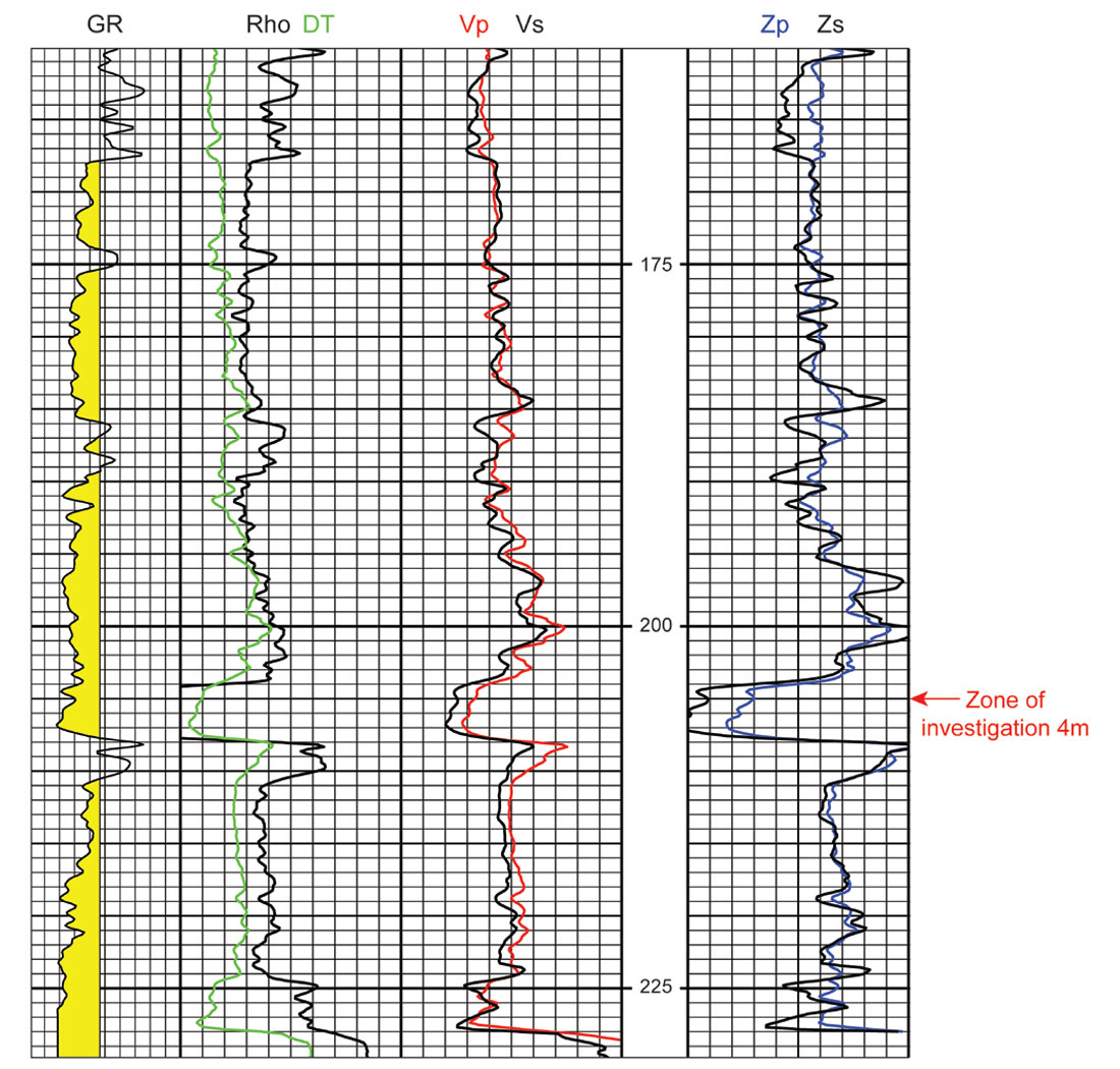
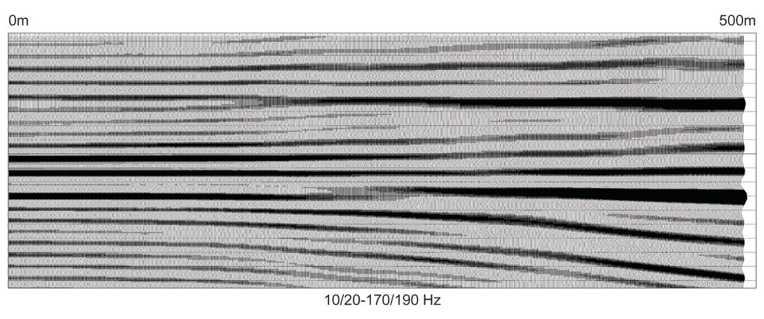
A synthetic AVO gather was created using an elastic-wave algorithm. The input elastic parameters were obtained from a well with P-wave sonic, S-wave sonic and density logs (Figure 1). The traces in the gather were generated at one-meter intervals over a range from 0m to 500m, and the wavelet was representative of real seismic in the area with a bandwidth of 10/20-170/190Hz (Figure 2). The well represents a shallow oil sands target, so each 10 meters of offset translates to approximately 1.5° incident angle at the zone of interest.

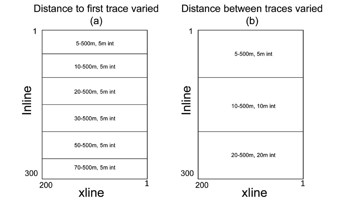
From this over-sampled dataset, variations and deficiencies were imposed to represent real examples of acquisition geometry. Pseudo 3Ds were created by repeating the same synthetic gather, but with slight variations in certain parameters. Figure 3a shows the synthetic 3D outline labeled by the distance to the nearest offset, which was varied from 5m (1°) to 70m (10°) (with a constant trace interval of 5m), for groups of 50 inlines; Figure 3b shows the same synthetic 3D geometry within which the trace interval was varied from 5m to 20m for groups of 100 inlines. For the second scenario, the nearest offset was also realistically adjusted to equal the trace interval. To reiterate, every CDP in both of these synthetic 3Ds represents identical geology with identical frequency content; the only parameters varied are those representing sampling. Indeed, the two scenarios created in these synthetic 3Ds reflect real acquisition sampling choices: the modeled variation of the distance to the nearest offset is representative of the distance between shot and receiver lines; the variation of the trace interval is dependent upon the shot and receiver spacing in a real survey.

Each synthetic 3D was input to identical AVO/inversion workflows. The two-term Fatti (Fatti et al., 1994) equation was used to derive P and S-reflectivity from the input synthetic gathers. The velocity model and background Vp/Vs equation were both derived from the well that was used to make the synthetic gathers, as were the impedance models. Depending on the modeling philosophy, the wavelet and scalars used for inversion of the reflectivities could be identical for each synthetic 3D, or they could be derived from the individual data volumes. In this study, they were derived from the individual data volumes, representing the very real influence of acquisition variations on parameter derivation and selection.

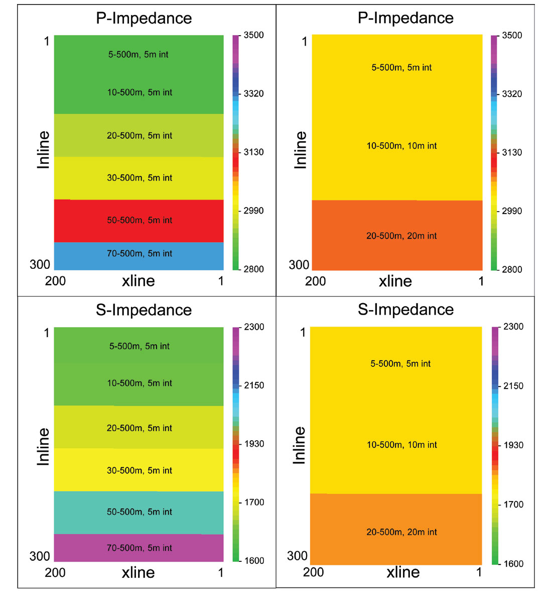
Figure 4 shows a time slice through each synthetic 3D survey at the target level for the resulting P-impedance and S-impedance derivations. Variations in impedance amplitude predictions are clearly seen corresponding to changes in the sampling parameters. The graphs in Figure 5 show these predictions quantitatively compared with the known P-impedance and S-impedance at the target zone in the well. It is obvious from these graphs that the accuracy of the impedance prediction is inversely proportional to the distance to the nearest offset, while the variation in trace interval has less effect on the impedance prediction (since models, wavelets and scalars have been derived from each synthetic volume independently, there is a slight shift between absolute values of impedance predictions derived from the separate volumes – the relative difference within each volume is the key measure).

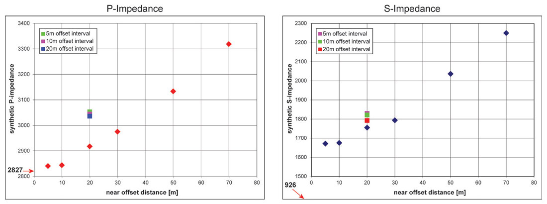
Even the nearest offset gathers were unable to estimate the S-impedance with as much accuracy as the P-impedance, but S-impedance is more difficult to estimate in any case, and the inverse trend between prediction accuracy and near-offset distance remains.

Figure 6 shows this conclusion in a different way with the impedance logs displayed at the same scale and sample rate as the predicted impedance traces. The arrows identify areas of comparison between the predicted impedance curve for the 5m near offset and the 70m near offset. Most would conclude that the impedance on the left (5m near offset) displays higher ‘resolution’ than the one on the right (70m near offset), so the somewhat surprising result is that the improvement in resolution is due solely to sampling, not frequency content, of the input data.

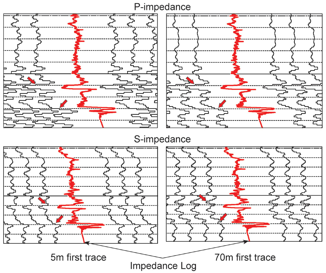
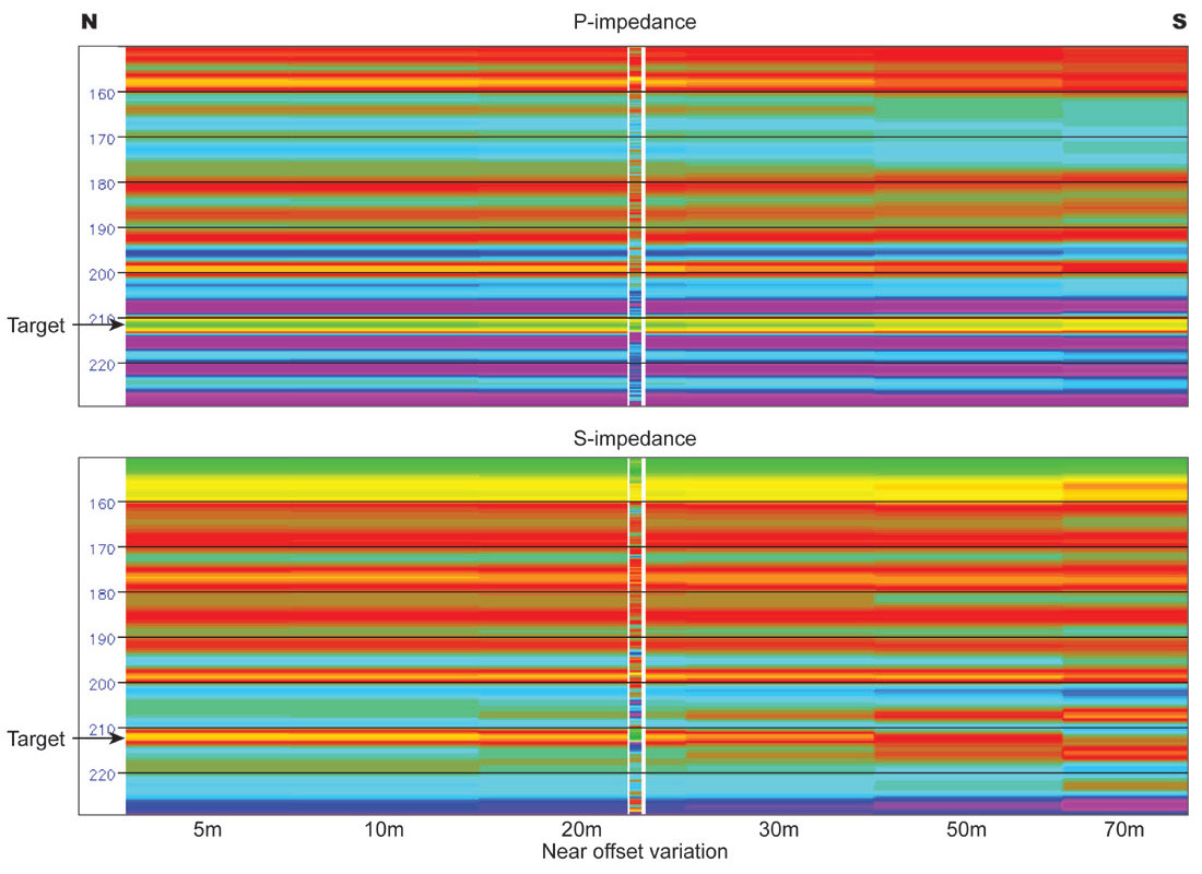
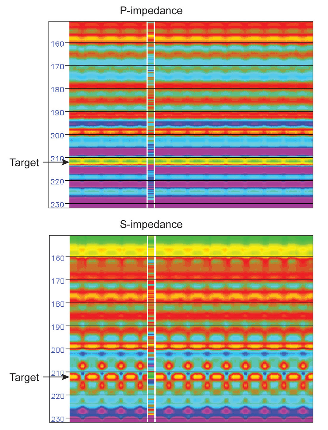
Figure 7 shows these inversion results along a ‘North-South’ line through the variable near-offset gathers, which cuts across each 50-line interval of constant parameters. If these traces are rearranged to represent a typical distribution of near-offset variation within a realistic 3D survey, an alarming footprint appears (Figure 8). (As expected, the presence of this footprint affects even the straightforward time-structure mapping of events on the conventional stack).

The results of this modeling exercise lead to the conclusion that near offsets are very important for accurate resolution and estimation of rock properties, as illustrated by the quantitative examples above. Near offsets, however, are the most expensive offsets to acquire with costs rising exponentially in proportion to near offset coverage. Hence the near offsets are the ones that are most often inadequately sampled in a real 3D seismic survey. Trace interpolation may be able to help. The real data examples in the next section illustrate the effectiveness of creating missing data using pre-stack interpolation.

Real Data Investigation

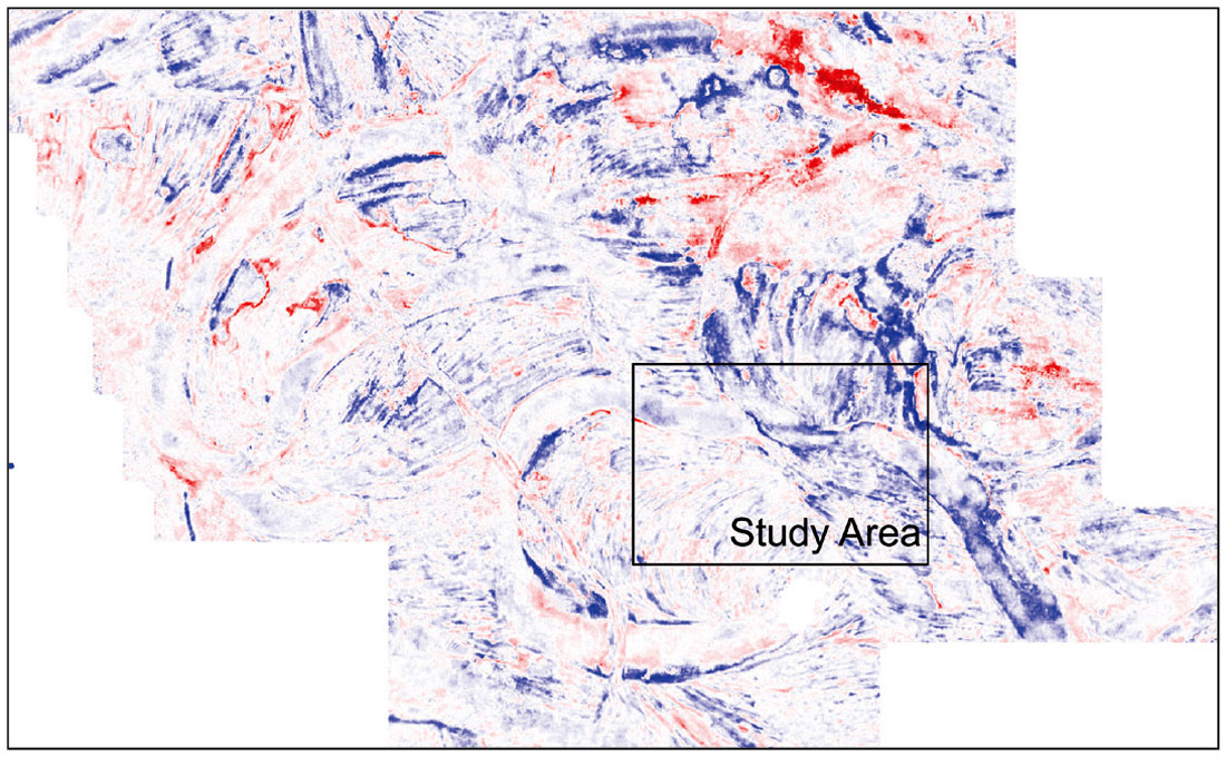
The real data incorporated in the study were a subset of the Nexen Long Lake South 3D seismic data shown on the map (Figure 9). The original acquisition geometry, which is quite dense compared to typical industry parameters for oil sands 3D seismic data, was used for the reference QI workflow and products. Two datasets were then created from the original by depopulating the acquisition geometry.

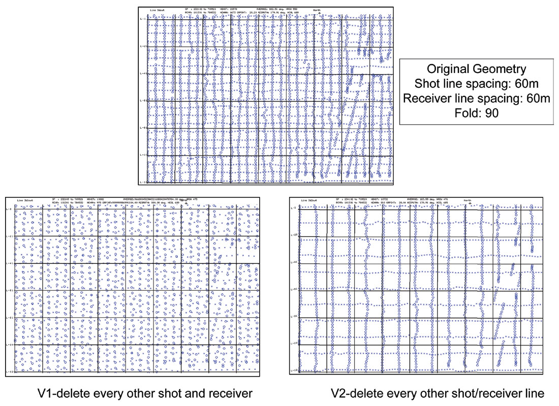
The first depopulated survey (V1) had every second shot and receiver station removed, doubling the trace spacing and creating a dataset with one-quarter the original fold. The second depopulated survey (V2) also created a dataset with one-quarter the original fold, this time by removing every second shot and receiver line, thereby altering the distance to the nearest offset. Figure 10 shows the shot and receiver locations for each of the test configurations. Each of the depopulated volumes was then interpolated using a pre-stack interpolation algorithm to recreate a version of the original data with its original fold restored. In addition, the original volume was also interpolated creating a volume with four times the original fold. In total, therefore, six real data volumes were processed and compared at all stages of the QI workflow. This work was done before the 5D algorithm for interpolation was widely offered (Weston Bellman, Wilkinson and Deere, 2010) and therefore, the interpolation algorithm utilized for this analysis was not 5D. All datasets were pre-stack time migrated after interpolation.

The QI workflow applied here incorporates pre-stack and post-stack analysis to derive multiple attributes from each of the input volumes. All parameters that were not seismic-data dependent were held constant across the workflows to ensure comparability between the test volumes. Parameters such as estimated wavelets and inversion scalars were derived independently from each volume, but within identical data ranges. Figure 11 illustrates comparisons between the derived P-impedance from each of the five additional volumes for comparison to that of the original acquisition geometry. All attributes were generated and compared in this way, and then were used separately to predict facies and fluids for each geometry and interpolation test dataset.

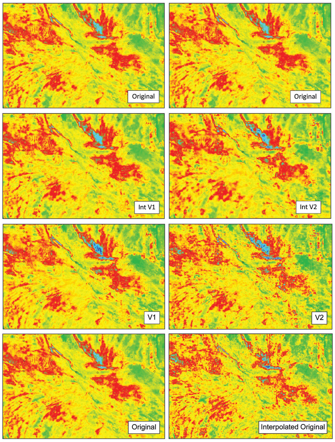
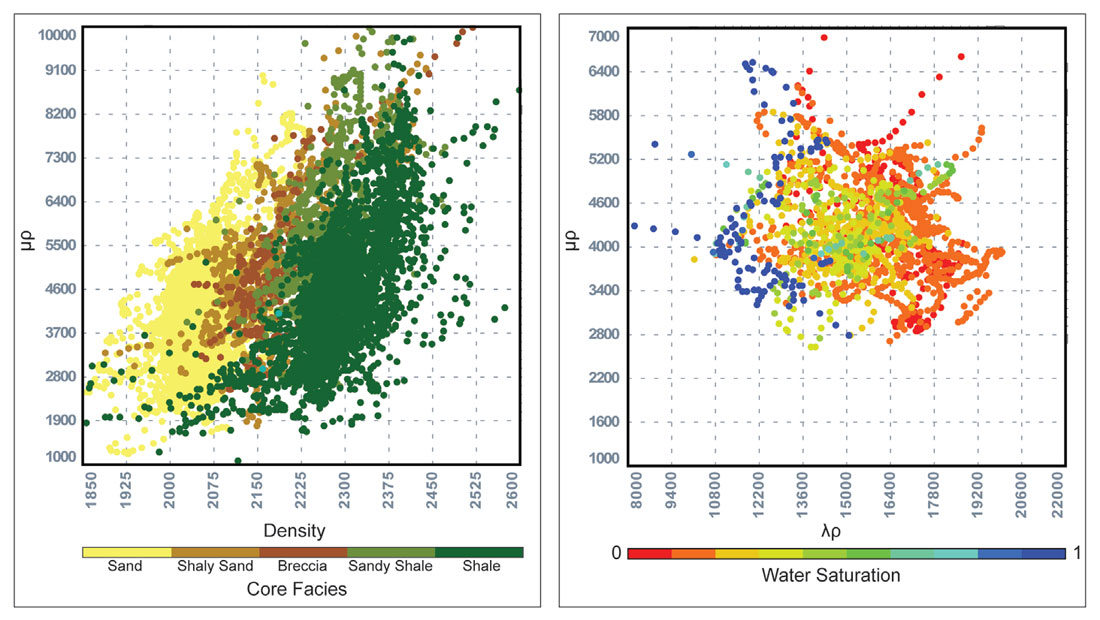
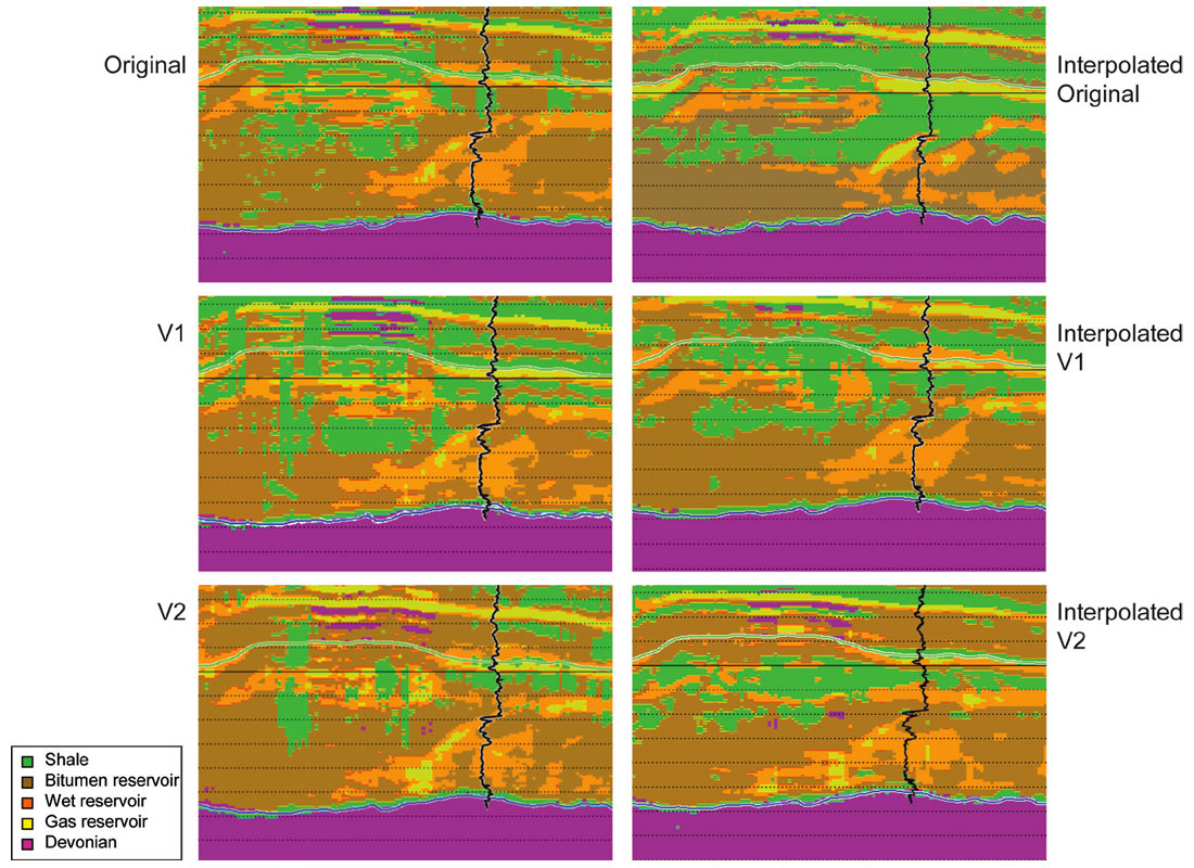
Templates for classification were determined using computed attributes from well logs. Figure 12 shows the two crossplots used to classify each set of derived attributes. The density vs. μρ crossplot shows effective separation between sand and shale, and the λρ vs. μρ crossplot highlights the further separation of sand facies into fluid types. Applying these templates to the appropriate attribute volumes resulted in the classified volumes shown in Figure 13 for each test dataset.

While general trends are all similar between classified volumes, comparisons of the details and the match with the gamma-ray log at one of the wells evaluated show significant variation. There is an obvious degradation in continuity and resolution (and accuracy) of the depopulated data versions (V1 and V2) compared with the original volume. Encouragingly, however, the interpolated decimated versions are both very close to the original, providing confidence in the integrity of the interpolated data. This similarity with the facies and fluids predicted by the original data is especially true for interpolated version 1. The less accurate interpolated version is the version that represented the decimation of near offsets (increasing the spacing between shot and receiver lines). Given the importance of the near offsets highlighted by the model analysis above, one can say that the interpolation did improve upon the results achieved without interpolation, but it is not perfect. Overall though, the best match at the well location is the interpolated original, which displays the best prediction of the shale thickness at the top of the reservoir zone and the gas that is present at the top of the sand. These empirical results imply that even well-sampled acquisition can be improved upon with a pre-stack interpolation.

Conclusions

This study highlights the need for careful consideration of seismic acquisition geometry for AVO applications. AVO and other quantitative interpretation processes rely on accurate measurements derived from pre-stack seismic data, and acquisition parameters can have a significant effect on the outcome.

The results of the modeling analysis conducted here highlighted the importance of near offsets to the accuracy of rock property predictions from seismic data. Given that near offsets are expensive to acquire, a project-specific modeling study that incorporates AVO behaviour may be warranted to determine the magnitude of uncertainty that can be tolerated, so acquisition parameters can be adjusted accordingly.

While acquisition of real data is always the ideal, in light of practical economic or environmental limitations, this ideal is never realized. In that case, the empirical results in the analysis described here lead to the conclusion that performing interpolation to fill in the gaps improves the final results; with the increasingly sophisticated methods commercially available today, even higher quality of predicted data is anticipated.

Some questions and ideas for additional investigation remain. The results in this study are specific to a particular modeled scenario and real data conditions. Would this type of detailed (and time-consuming) comparison be necessary in every case or are there ‘shortcuts’ to determining the relative benefits of acquisition vs. interpolation? In this type of comparison, in spite of many objective measures of success, there are certainly subjective factors that may influence the final assessment. Are there definitive objective measurements? And finally, is there a possibility for the eventual development of ‘least-effort’ guidelines in acquisition design – some type of combined acquisition and interpolation function that minimizes cost and maximizes quality? I look forward to continuing the discussion.

Acknowledgements

I would like to thank Key Seismic Solutions for preparing the model and real data for analysis, and acknowledge the data contributions by Nexen Energy ULC.