AVO Feasibility and Reliability Analysis in the Presence of Random Noise

Abstract

AVO inversion provides a cost effective means for predicting elastic parameters and rock properties of the earth. However, the results of AVO inversion are sensitive to noise. For some acquisition, geometries and noise levels predictions from the AVO inversion may not be reliable. By studying the influence of random noise on the AVO inversion problem, insight can be gained as to where AVO inversion might be applicable, or just as importantly we may gain insight as to where AVO will not be applicable. The primary factors influencing the reliability due to random noise are: the prestack signal-to-noise ratio, the fold, and the range of angles available for the AVO inversion. For Gaussian independent noise, the effect of these factors can be understood by studying the data covariance matrix.

Prior to investing the time and effort in a large AVO study, a feasibility study can be performed to understand whether the seismic data is suitable for AVO inversion. Further, after having performed an AVO inversion, it is important that the interpreter incorporate reliability quality controls into their interpretation so as to avoid drilling an anomaly created by noise or the acquisition geometry footprint.

Introduction

Over the last decade, one of the significant trends in geophysics has been the increased use of AVO inversion to help better characterize the reservoir in seismic exploration and development. This increased use of AVO inversion is in part due to changing the AVO interpretation paradigm from generating and interpreting AVO anomaly stacks to generating elastic parameter estimates, and then interpreting these estimates in the context of our knowledge of rock physics. The approach outlined by Goodway et al. (1997) is an example of this.

As the predictions from AVO become more quantifiable, it is also important to quantify the uncertainty associated with AVO predictions. In predicting rock and fluid properties from the elastic parameter estimates, the interpreter needs to understand how much he or she can trust the results of the AVO inversion and therefore know how much confidence one can place in their rock and fluid property predictions. The quantification of this uncertainty is a complex area and the techniques will evolve over the coming decade. This paper looks at one aspect of this issue. How should we quantify the reliability of AVO inversion in the presence of random noise? A methodology is introduced to estimate the reliability in the presence of Gaussian independent noise. It is shown that this can be done prior to a project as a feasibility study or incorporated as part of the AVO inversion as reliability quality controls.

To develop this methodology, the linearized AVO approximation is first introduced. Bayes theorem is then discussed as a way of studying the probability and uncertainty of the elastic parameter estimates from the linearized AVO approximation in the presence of random noise. It is then shown by way of example that for data with typical signal-to-noise ratios, the results of the three parameter AVO inversion are generally not reliable. That is, the uncertainty of the estimate is greater than a significant fraction of the estimate itself. It is shown that by introducing a priori information the estimates will appear to have greater reliability, but at the expense of potentially introducing incorrect information into the problem through the constraints. The covariance matrix is introduced as a simple means to estimate the reliability of the AVO parameter estimates. To validate this approach, a modeling study is performed to compare the estimates of reliability with the actual reliability. Lastly, a data example is shown where the reliability estimates are used to help identify reliability issues in the AVO parameter estimates.

Theory

Amplitude variation with offset

Elastic parameters may be estimated by inverting a linearized approximation of the Zoeppritz equation such as the following approximation developed by Aki and Richards (1980)

where α, β, ρ, γ respectively are the average P-wave velocity, S-wave velocity, density and the ratio of S-velocity to P-velocity across the interface. The variable θ is the average angle of incidence and Δα, Δβ, Δρ are the changes in P-wave velocity, S-wave velocity and density.

If θ and γ are considered to be known apriori, equation (1) may be solved using linear inverse techniques. Equation (1) may be written more succinctly in matrix notation

where G is the linear operator, m the unknown parameter vector and d the input data vector. The parameter vector is composed of the density, P-and S-wave velocity reflectivity attributes. These are called reflectivity attributes since they share the same mathematical form as reflectivity but not the same physical significance.

Since the data is recorded as a function of offset, raytracing must be done to transform the functional dependence of the data from offset to average angle of incidence. The linear operator G is completely determined by the initial model; γ, the average angle of incidence θ and the acquisition geometry. Errors in these operations and assumptions will lead to systematic errors in the reflectivity attribute estimates.

Bayes theorem and uncertainty

Bayes’ theorem provides a theoretical framework to make probabilistic estimates of the unknown reflectivity attributes m from uncertain data and a priori information. The resulting probabilistic parameter estimates are called the posterior probability distribution function. The Probability Distribution function (PDF) written symbolically as P(m|d,I) indicates the probability of the parameter vector m given the data vector d (offset dependent reflectivity) and information I. Bayes’ theorem, which can be expressed as

calculates the PDF from the likelihood function P(d|m,I) and a priori probability function P(m|I). The denominator P(d|I) is a normalization function which may be ignored if only the shape of the PDF is of interest

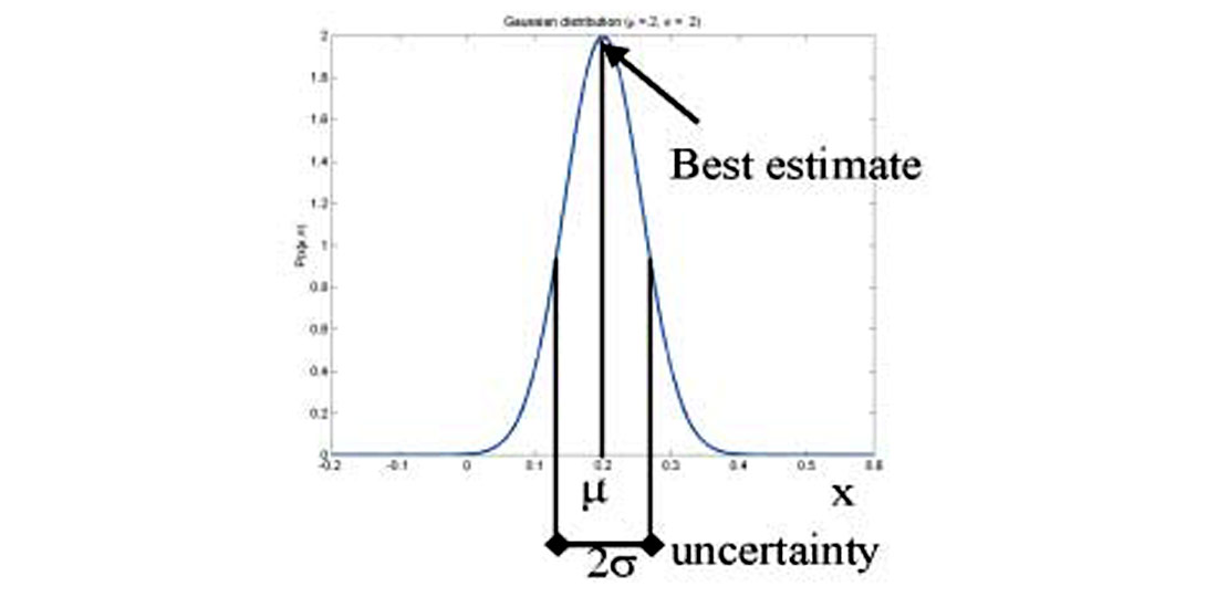
The most likely estimate occurs at the maximum of the PDF. The uncertainty of the parameter estimate is proportional to the width of the PDF.

To simplify the analysis of equation (4) it will be initially assumed that the prior probability distributions are uniform. In this case the Bayesian inversion is equivalent to maximum likelihood inversion. To simplify the analysis further, it is assumed the noise is independent and Gaussian. In this case the likelihood function may be written as (Sivia, 1996)

where σ² is the variance of the noise. Under these assumptions this optimization problem is equivalent to least squares.

For AVO inversion, because of the small number of parameters solved for, it is possible to visualize the PDF. If the parameter vector m had only one element, the PDF would be a Gaussian function (Figure 1). The most likely solution would be where the probability distribution is at the maximum. The uncertainty would be proportional to the width of the distribution. Since this is a Gaussian distribution, standard statistical parameterizations such as standard deviation or variance can be used to characterize the uncertainty.

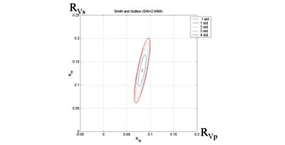
If the parameter vector m had two elements, the PDF would be a bivariate Gaussian function and an equi-probable solution would be an ellipse. This would be the case for the two term Fatti et al (1994) approximation, Shuey (1995) approximation and the Smith and Gidlow approximation (1987). Figure 2 shows the probability distribution solved for the Smith and Gidlow approximation, for a hypothetical reflector with a signal to noise ratio of 2. Each contour represents an equi-probable solution. In this example, the most likely solution occurs for the smallest contour ellipse or maximum probability at R_Vp=0.06 and R_Vs = 0.13.

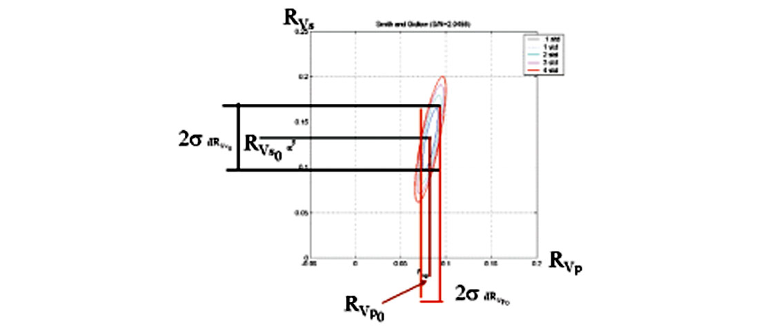
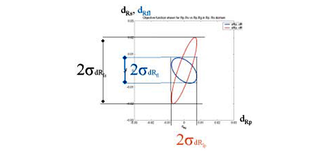
If we are interested in the uncertainty of the R_Vp estimate then we would have to know the one dimensional probability distribution for R_Vp. In calculating this we have no interest in the S-impedance reflectivity. The S-impedance reflectivity probability must be marginalized using

The uncertainty will be related to the total width of the ellipse projected onto the appropriate axis. Figure (3) shows this projection and it is evident that that S-velocity reflectivity will have greater uncertainty than the P-velocity uncertainty.

The bivariate Gaussian distribution

is described by a 2 by 2 covariance matrix . The physical significance of the covariance matrix will be discussed in greater detail in a later section.

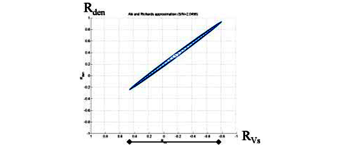
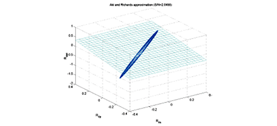
For the case of equation (1) there are 3 parameters so the PDF is a multivariate Gaussian function where an equi-probable solution is an ellipsoid. Typically the ellipsoid is quite elongated (Figure 4). Non-physical solutions, such as those in which the reflectivity has a magnitude greater than 1, are evident. Figure 5 shows one of the faces of the 3d cube shown in figure 4. It is evident that since the ellipsoid is so elongated that the uncertainty of both the S-velocity and density reflectivity will large. This is also true for the P-velocity reflectivity.

Constraints

Up to this point it has been assumed that unknown reflectivity attributes are uniformly distributed. As seen in the last section, this allows for non-physical solutions. Constraints can be used to eliminate them. One way of doing this is to place bounds or limits on the a priori distributions so the reflectivity magnitude must be less than one. This reduces the solution space and uncertainty. However, for noise levels typical in real data, the parameter estimates are still not accurate enough to make reliable predictions. Additional constraints must be employed to reduce the reflectivity attribute uncertainty to acceptable levels. This is at the expense of potentially introducing theoretical error arising from incorrect assumptions into the inversion.

For example, Smith and Gidlow (1987) suggested using the Gardner et al (1973) equation

to constrain the solution. In terms of reflectivity, equation (8) is

which defines a plane in the 3d solution space. Using Bayes theorem, the solution will be the intersection of this plane and the 3d ellipsoid (Figure 6). This constraint greatly reduces the uncertainty but at the expense of effectively removing one of the variables. The density reflectivity is no longer an independent variable. The inverse problem now only has two parameters where the probability distribution of these variables is the Bivariate Gaussian distribution described previously.

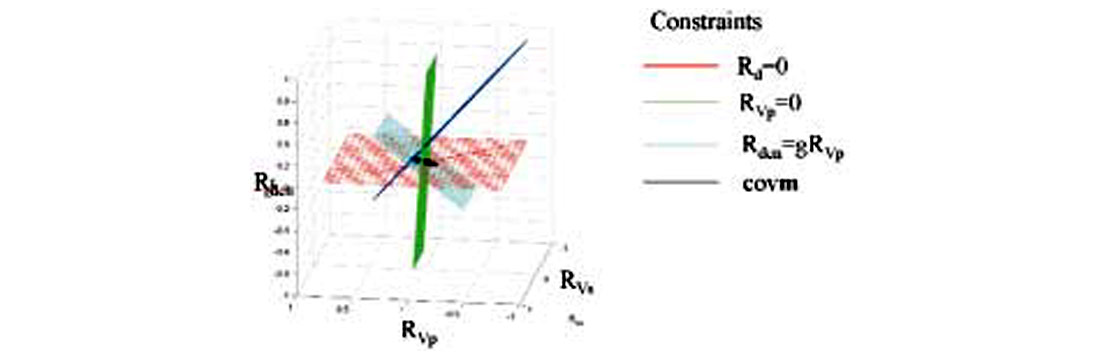
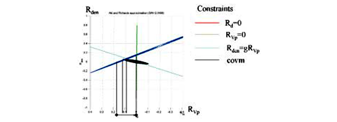
Both the Fatti and Shuey reformulations of equation (1) are often solved using only the first two terms. This is equivalent to setting the third term to zero. For Shuey’s equation this sets the P-velocity reflectivity to zero and for the Fatti equation this sets the density reflectivity to zero. Figure 7 shows the application of these different constraints in 3 parameter solution space. In each case the optimal solution is the intersection of the plane with the misfit ellipsoid. Each constraint results in a slightly different optimal solution (Figure 8). The solution will be as good as the prior knowledge leading to the constraint. Determining which solution is most realistic involves answering the question, “is it more realistic that the velocity reflectivity is zero, that the density reflectivity is zero or that the Gardner equation holds?” By introducing the constraint, the uncertainty has been reduced but at the expense of introducing error arising from the correctness of the a priori information.

Covariance Matrix

In practise, most AVO inversion being done in the industry today is using some form of two term constrained inversion. This being the case, the rest of the paper will consider how to quantify the influence of noise for this particular inversion problem. In the previous section, it was shown that the probability distribution for the two term AVO inversion could be described by a bivariate Gaussian distribution. In turn the bivariate Gaussian distribution is uniquely parameterized by a 2 x 2 covariance matrix. The inversion problem under these assumptions is equivalent to least squares inversion.

It can be shown for least squares inversion that the uncertainty of the parameter estimates is described by (Menke, 1994)

where C_d is the data covariance matrix and estimates the parameter reliability. Equation (10) suggests that the data covariance matrix is only a function of the prestack noise variance σ² and the linear operator G.

The diagonal elements of the data covariance matrix are the variance of each of the parameter estimates. The off diagonal elements show the amount of correlation between the variance of two variables. The standard deviation, which is the square root of the variance, is a measure of reliability of each variable. In the case of the two term Fatti et al (1994) equation, the data covariance matrix is

where σ_Rp is the standard deviation of the P-impedance reflectivity, σ_Rs is the standard deviation of the S-impedance reflectivity and σ_RpRs the covariance between the P- and S- impedance reflectivity.

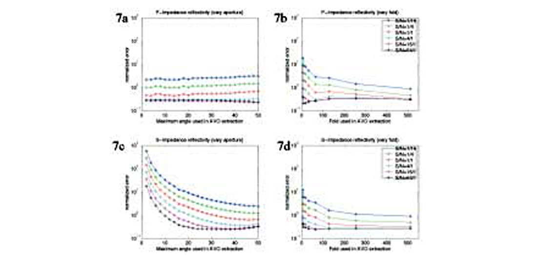
In studying the covariance matrix (equation 10) it is sometimes instructive to separate the influence of the prestack noise σ and the inverse of the normal equations, [G^TG]^-1. The prestack noise acts as a scalar, the more noise the greater the uncertainty. The normal equations are solely determined by the acquisition geometry and Vp/Vs ratio. The influence of different acquisition parameters such as maximum and minimum offset can be studied using equation (10). Figure 9 shows the results of such a study. In the first set of examples (Figure 9a,b,c) the fold was held constant, while the angles used in the AVO inversion were varied. In Figure 9a the maximum angle included in the AVO inversion was varied while the minimum angle was held constant at zero. The uncertainty in the S-impedance reflectivity decreases as the maximum angle used increases in a nonlinear fashion. For small maximum angles, increasing the angle range by a small amount greatly decreases the uncertainty. For large maximum angles, the effect of increasing the angle range by a small amount is less noticeable. Because of this, for typical prestack S/N ratios, it is desirable to have a minimum maximum angle of at least 20 degrees and preferably 30 degrees. The standard deviation of the P-impedance, unlike the standard deviation of the S-impedance, seems to be insensitive to the maximum angle used.

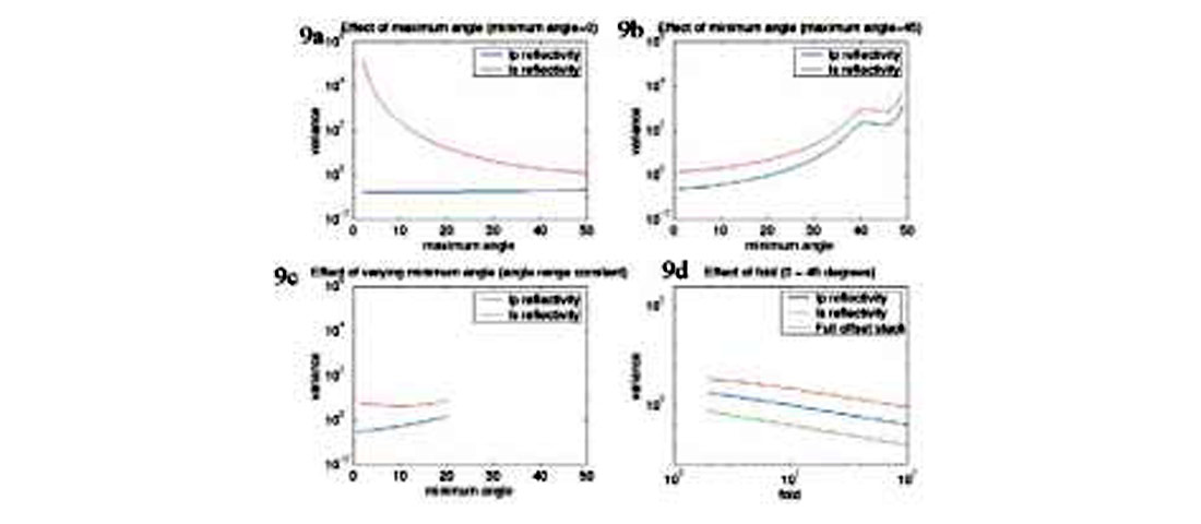
The influence of changing the minimum angle while holding the maximum angle constant is shown if Figure 9b and the case of varying the total range of angles used in the AVO inversion shown in Figure 9c. This suggests that influence of the minimum and maximum angle can be described by one parameter, the useable angle range or aperture.

Lastly the effect of fold is considered. In this analysis the angle range is held constant. In Figure 9d it is observed that if the fold increases, the reliability of the estimates increases. This is due to the fold effectively increasing the poststack signal to noise ratio and thereby increasing the reliability of the estimates. This is an interesting observation since this suggests that one way of increasing the S-impedance reflectivity reliability is to increase the fold acquired in data acquisition.

Fluid stack

In order to analyze two reflectivity sections simultaneously, interpreters often look at linear combinations of reflectivity attributes. The fluid stack (Smith & Gidlow 1986), (Fatti et al, 1994) is an example of this. The Rp and Rs section when cross-plotted should cluster along a line whose slope is defined by the mudrock relationship (Castagna et al, 1985) and the background Vp/Vs ratio. Significant departure from the line (cluster) may indicate the presence of gas. The fluid stack is calculated by

where ΔF is the Fluid stack and m is the slope of the mudrock line. This simple linear relationship can be written in matrix notation using the transform matrix T to map the P-and S-impedance reflectivity variables to Fluid stack and P-impedance reflectivity. Knowing the variance of the P and S impedance reflectivity, and the transform matrix T, it is a simple matter to calculate the variance of the fluid stack using

where C_’d is the covariance matrix after the transformation. Figure 10 shows the variance before and after the transformation where the original variables P-and S-impedance reflectivity variance are transformed to the P-impedance reflectivity and fluid stack variance. It is interesting to note that the fluid stack has less variance than the S-impedance reflectivity. This is due to the fact that the covariance term σ₁₂ is significant and negative.

Feasibility and Reliability Analysis

The reliability of the AVO attributes can be calculated using the above methodology prior to doing an AVO analysis, as a feasibility study, to understand whether the proposed seismic survey has the required fold and aperture to get useable results. Some sort of estimate of the prestack noise level is needed to do this analysis. This analysis could also be performed as part of the AVO inversion to provide reliability quality controls to help with the interpretation of the AVO attributes. In this case the prestack noise level can be estimated by calculating the misfit of the model to the data. To validate that the above covariance matrix methodology gives reasonable estimates of reliability a modeling study was performed testing the key variables identified above.

Modeling study

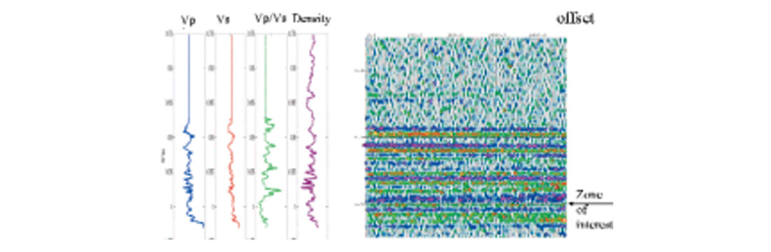
A well log from western Canada which had Vp, Vs and density information was used to generate a primaries only forward model using the Zoeppritz equation and ray tracing (Figure 11). The model was designed to test the effect of fold, aperture, and prestack signal-to-noise ratio separately. To do this, the low frequency velocity trend of the Glauconite gas well was modified such that over the window from .88 to 1.1 seconds, the angle of incidence is roughly constant for each offset. This allowed the fold to be varied independently of angle of incidence in the testing. The Vp/Vs ratio and density curves were retained from the original log.

Two sets of gathers were created. The first set of gathers was designed so that 25 separate AVO extractions could be performed over different angle ranges while keeping the fold constant at 64 and the minimum angle constant at zero. The maximum angle was allowed to vary from 2 to 50 in 2 degree increments. Noise was added to these gathers with the following signal-to-noise ratios: 64/1, 16/1, 4/1, 1/1, 1/4 and 1/16. To understand how the extraction behaved at the end points, one set of gathers had no noise and another set was all noise. This resulted in 200 permutations (25 different angle records times 8 noise levels).

The second set of gathers was designed such that the angle range in the AVO extraction could be held constant (0 to 45 degrees) while the fold was allowed to vary over the following range: 4, 8, 16, 32, 64, 128, 256 and 512. The same noise levels were combined with this data resulting in 64 permutations (8 different fold records times 8 noise levels).

AVO extractions were then performed on both these sets of records to get estimates of P and S-impedance reflectivity using the 2 term Fatti equation. A simple low frequency velocity model was used to ray trace the data. The Vp/Vs ratio was smoothly varying. These were constructed, as one would normally do in performing an AVO inversion on real data.

Modeling Results

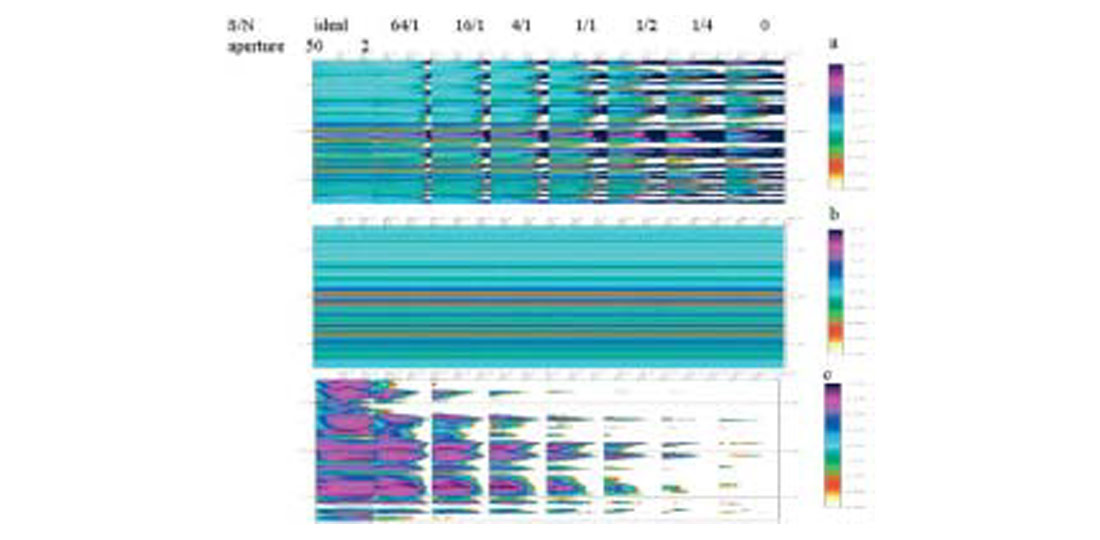
The top panel of Figure 12 shows the estimate of S-impedance reflectivity when the angular range is varied. This is compared to the ideal zero offset S-impedance reflectivity displayed using P-wave travel time (Figure 12, middle panel). The fractional error (figure 12, bottom panel ) is calculated using

where IA is operation of taking the instantaneous amplitude (Taner, 1977). Figure 13 shows the estimate of the fractional uncertainty of the S-impedance reflectivity predicted by the covariance matrix. This agrees well with the ideal fractional uncertainty (Figure 12c) calculated using equation (14).

The prediction of uncertainty was then compared to the actual misfit numerically. The actual misfit for both the P- and S-impedance reflectivity attributes was calculated over a 100 millisecond window, centered on 0.950 seconds and displayed in Figure 14. These measurements of the actual uncertainty are consistent with the predictions made by the covariance matrix in the preceding section (Figure 9). The P-impedance reflectivity is insensitive to angle range while the S-impedance reflectivity is strongly sensitive to aperture in the same manner as suggested by Figure 9a. It is interesting to note that at high angle and fold the fractional error actually increases. This is due to error introduced by the a priori information used to constrain the problem.

Data Example

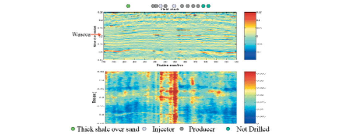
To illustrate the use of reliability predictions on real data, a fluid stack (Figure 15) is shown for a seismic line shot over a heavy oil field undergoing steam injection. Modeling studies suggest the fluid stack should show an anomaly where the reservoir is at elevated temperatures. The line was shot while production was ongoing. As a result there is considerable noise from the pumps causing reliability issues with the reflectivity attributes at several places along the line. The fluid stack shows an anomaly at the base of the Waseca sand that corresponds well with most of the producing wells and injectors. However, the injector at station 280 does not show an anomaly. It is interesting to note that the standard deviation of the fluid stack at station 280 is several orders of magnitude greater than the fluid stack estimate. This suggests that the fluid stack attribute is unreliable at this point and the prediction should be ignored. With the incorporation of the reliability information, the fluid stack is consistent with the geologic control. By knowing where the AVO estimates are reliable and just as importantly where they are less reliable, greater confidence can be placed in the AVO interpretation in general.

Conclusions

It has been shown that in the presence of noise, constraints are needed to make the reflectivity attribute estimates for the linearized AVO inversion, more certain. This comes at the expense of potentially introducing theoretical error into the problem. The correctness of different approximations published in the literature can be viewed in terms of how geologically plausible the used constraints are.

In the case of Gaussian independent noise, equation (10) may be used to predict the reliability of the reflectivity attribute estimates. In this case, the reliability is only a function of the prestack noise and the line geometry. The variance of the parameter estimates are directly related to the variance of the prestack noise. Increasing the fold or the number of traces used in the analysis increases the reliability by increasing the poststack signal-to-noise ratio. The greater the range of angles used in the AVO inversion the more reliable the results. This can be accomplished by incorporating larger maximum angles or smaller minimum angles. There are practical limits to this due to processing limitations and theoretical concerns such as excluding the critical angle and the appropriateness of the constraints.

Equation (13) using the transform matrix provides a convenient way to understand the reliability of different reflectivity attributes. It has been shown that the P-impedance reflectivity and the fluid stack are more reliable than the S-impedance reflectivity.

The covariance matrix can be created before or as part of the AVO inversion. If it is done before as part of a feasibility study, it can help determine if the seismic data set is suitable to run AVO on. If it is run as part of the AVO inversion, the quality controls that are generated can be used to help appropriately weight the AVO reflectivity attributes into the overall interpretation.

It is important to note that this paper has not considered the impact of coherent noise and systematic errors such as incorrect scaling. Further the linearized AVO model (equation 1) is itself an approximation of the more complex reality. The implication of this is that the reliability estimate will be more optimistic than if these other issues were included in the analysis. The reliability estimates that are generated must be viewed as an upper limit on what the actual reliability might be. This being the case, the reliability estimates are still valuable in that they identify problem areas in the survey due to acquisition geometry and noise.

Acknowledgements

The authors acknowledge A.O.S.T.R.A and Husky for permission to publish the data example. In addition, the authors thank Jan Dewar, Satinder Chopra and Yongyi Li for their critical comments.