Aliasing for the Layperson

Introduction - Aliasing in Everyday Life

Examples of aliasing can be observed in western movies by watching the motion of stagecoach wheels. As the stagecoach starts to move, we observe its wheels rotating in the expected forward direction. As the stagecoach speeds up, we see that the wheels appear to rotate in the opposite direction to the initial one. We realize that this phenomenon happens because the movie consists of a number of frames or “digital samples”. With the wheels’ acceleration, the digitized succession of frames will show the spokes appearing to move in the opposite direction to the actual direction of the wheels’ rotation. This occurs because the movie camera has undersampled the wheels’ motion. Similar effects in real life occur when one watches a helicopter blade as it speeds up. The blades’ apparent motion is sampled too slowly by our brain to detect the actual motion, and they may appear to have a slower rate of rotation than the true rotational speed.

Strobe Light Experiments, Sampling, and the Nyquist Frequency

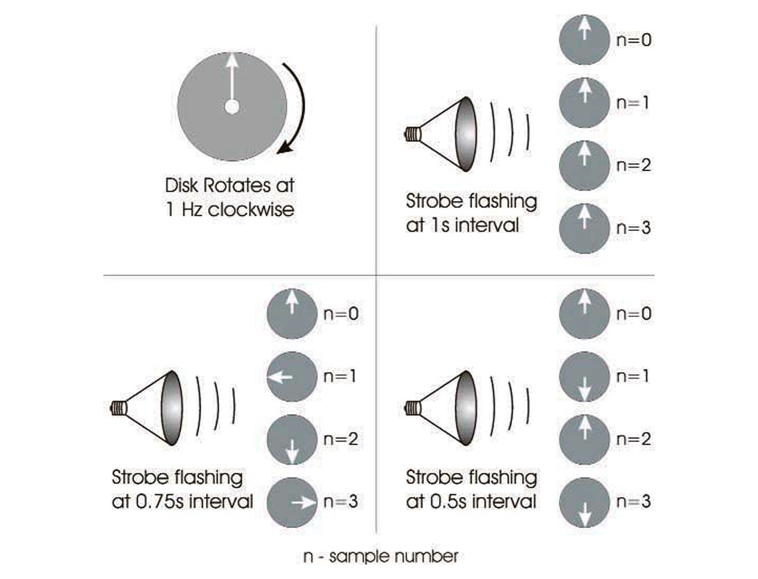
An illuminating example of aliasing and the sampling concepts comes from a physics experiment in which we attempt to detect the angular speed of a rotating disk by the use of a flashing strobe light. We note that if the frequency of the strobe flashes coincides with the frequency of the disk’s rotation we can “freeze” the motion of a point on a disk. However, the freezing of a point on the disk also occurs if our disk’s rotational frequency is at some integral multiple of the strobe light’s frequency. For example, consider a disk in Figure 1 that is rotating in a clockwise direction at 1 cycle per second. We mark a point on the disk with an arrow to indicate its position. If we set our strobe flashing at periods of 1, 2, 3 s (i.e. at frequencies of 1, 1/2, 1/3 Hz), we will see the arrow appear at the same location. The highest strobe frequency, which allows the arrow to be frozen, is the sampling frequency of 1 Hz. If we set the strobe light to flash slightly faster than once per second, we see that the arrow appears to move in the counterclockwise direction. For example, if the strobe flashes every 0.75 seconds, we first see the arrow appear at -90 degrees (or +270 degrees), then at 180 degrees, and then 90 degrees from its initial vertical position. If we set the strobe light to flash every 0.5 s (2 Hz) we will see the arrow alternate between pointing vertically upward and downward. The strobe light samples the disk’s position twice every cycle. Setting the strobe light to have a sampling rate of 0.5 s, we can detect the 1 Hz rotation of the disk. For a strobe light sample interval of 0.5 s, the maximum definable frequency of disk rotation is 1 Hz. If the disk rotates any faster than 1 Hz, then we must use a finer sampling interval to detect it. This maximum measurable frequency for a given sample interval is known as the Nyquist frequency, and was named in honor of Dr. Harry Nyquist, an American physicist and engineer.

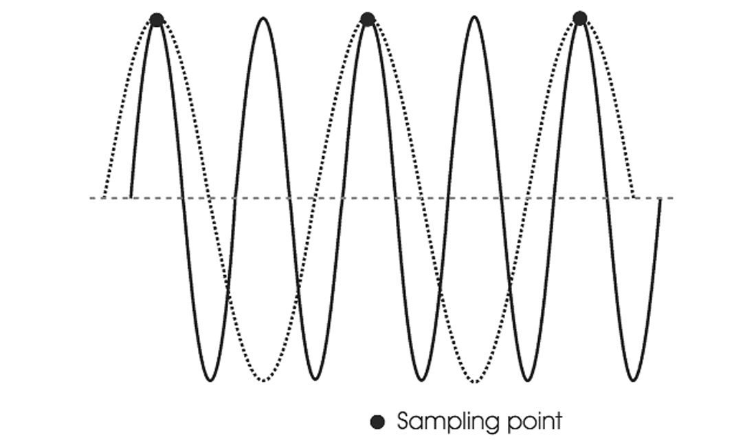
Through Fourier analysis, any seismic signal can be decomposed into weighted sums of sines and cosines. By analogy with the rotating disk and strobe light, it is useful to note that we must sample the sine wave at least twice every cycle (sampling a peak and a trough) in order to detect its frequency. Figure 2 (adapted from Cary (2001)) shows the consequence of inadequate time sampling - we see a sinusoidal wave at a lower frequency. For example, if we measured the sine wave only once per cycle, we would measure the same sample value and it would appear as a DC signal.

In other words, if our sample interval is set at Δt, then the Nyquist frequency is given by :

Digital field recording of seismic signals converts the continuous motion of seismic vibrations as recorded by seismometers or hydrophones into a sequence of digital values. If we set a sample interval at a typical value of 2 ms, the Nyquist frequency is 250 Hz. Frequencies above 250 Hz in our signals will be aliased or recorded as apparently lower frequencies just as in the case of the wagon wheels or rotating disks which appear to be rotating in the wrong direction. Therefore, in order to avoid such problems, the anti-alias filter in the recording truck must be set to electronically filter out frequencies above 250 Hz in analog signals prior to digitization. This is a necessary step taken in seismic recording to avoid the temporal aliasing encountered by digital sampling of time series.

Spatial Aliasing

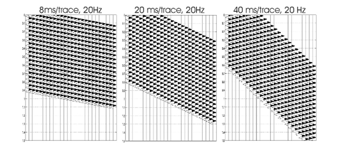
There is an analog anti-alias filter in time sampling. Unfortunately, the same type of anti-aliasing filter does not exist for spatial sampling where we record with a discrete number of receivers. To appreciate the problem of spatial aliasing, we refer to some plots taken from Seismic Data Processing by Hatton et al. (1986). Figure 3 shows a set of dipping sinusoidal traces with a frequency of 20 Hz. That is, their period is 50 ms. In the left set of traces in Figure 3, we see sinusoidal traces with a stepout of 8 ms/trace such that the traces are dipping to the right. With delays of 20 ms/trace, the traces still appear to dip to the right. However, if the traces are delayed by 40 ms per trace, they now appear to be dipping to the left. Aliasing has occurred. Why does this happen? Recall that temporal sampling required that we sample a sinusoid twice every period. In other words, adjacent samples must be less than half a period apart. If we observe the spatial samples of adjacent traces at a given time, we note that aliasing occurs when the delay between traces (40 ms in the aliased example) is greater than half of the period, which in this case is 25 ms. The increased stepout per trace causes the aliasing. The stepout difference between the aliased and unaliased sections could occur for at least two reasons. If the events represent reflections, it may be due to the physical dip of the reflector. Alternatively, the stepout difference between the aliased and unaliased sections could be due to the spacing between geophones. In other words, this could occur if the geophone spacing in the aliased section was twice that in the unaliased section. Our spatial sampling of the wavefield by geophones could be too sparse in the aliased case.

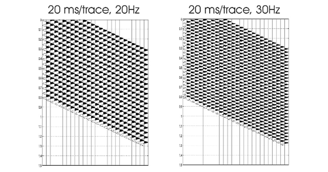
The example in Figure 3 suggests that spatial aliasing could be caused by steep dip and sparse geophone spacing. Spatial aliasing is also affected by the temporal frequency of our signals. Figure 4 is another example from Hatton et al. (1986) that demonstrates this phenomenon. The left part of Figure 4 shows the unaliased case of 20 Hz sinusoids having a stepout of 20 ms/trace. If we change these sinusoids from 20 Hz to 30 Hz and maintain the same stepout per trace, we can also see an apparent dip to the left instead of an apparent dip only to the right. Aliasing has occurred due to an increased frequency.

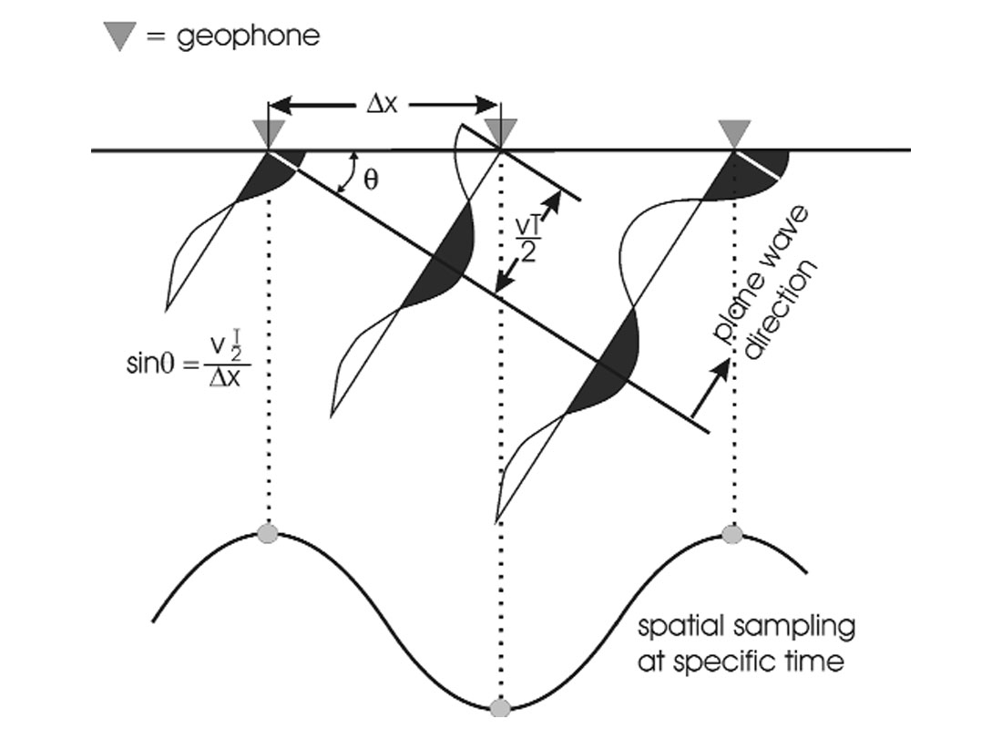
To further analyze spatial aliasing, let us consider the situation in Figure 5 of an emerging plane wave traveling upward with a velocity v and hitting the surface at an angle θ. Let the spacing between geophone elements be Δx. In order to avoid aliasing, we recall that the time stepout between adjacent traces should be at most half of the period of the sinusoid which we denote by . If we examine Figure 5, we see by inspection that sin θ = .

We can relate this analysis of a transmitted plane wave to the case of a reflected wave if we recall the “exploding reflector” model for zero offset data described by Loewenthal et al. (1976). Loewenthal et al. pointed out that reflections resulting from 2-way travel from a point to a reflector and back to the same point can generally be described by a wave experiencing 1-way travel from the reflector to the source point if the wave travels at half the velocity of the medium. Therefore, we can consider the emerging plane wave in Figure 5 to be a reflected wave if we replace v with in the previous expression for sin θ, where V is the seismic velocity of the medium. We now have the expression that gives the limiting values to avoid aliasing. If the frequency of our sinusoidal waves is fixed at f = , then the geophone spacing, Δx, must satisfy the following condition, which we obtain by substituting for the medium velocity and period in the previous expression, also given by Yilmaz (2001).

Equivalently, if our geophone spacing is held constant, we can say that to avoid aliasing we must limit the temporal frequencies or the dip by the above expression. We should note that equation (2) is somewhat simplified in that it is derived for a zero-offset section and is generally not the relationship for geophone spacing in typical shot gathers. For the more general cases, the reader should refer to pages 21-23 of Cordsen, Galbraith, and Pierce (2000), or to an upcoming paper by Cary and Li (2001).

In practical terms, we need to be aware of how this expression affects our survey design and the temporal frequencies that we can hope to image in our seismic experiments. We realize that aliasing can be avoided in time by electronically filtering out the high frequencies above the Nyquist frequency prior to digitization. How can we avoid the effects of spatial aliasing?

If we examine equation (2), we see that one way to avoid aliasing is to design the seismic survey with closely spaced geophone groups so that equation (2) is satisfied. This requires that we have some knowledge of the wave’s velocity, the steepest dip of the reflecting horizons, and the largest usable temporal frequency. Of course there is a practical tradeoff between the expense of a survey (which increases with decreasing group spacing) and our desire to avoid spatial aliasing.

Sometimes we do not have complete knowledge of steepest dips and minimum velocity a priori, and we are dealing with data that have been recorded with geophone spacings that allow aliasing of high frequency events. What do we do in such situations? Some remedies to this problem are outlined by Yilmaz (2001). One approach would be to decrease the temporal frequencies by low pass filtering of our data. This approach may suffice if we are not concerned about the resolution of thin beds. However, we realize that removing the high frequencies will increase the effective wavelength and degrade resolution. Another approach would be to decrease the apparent dip of our events by time shifting; however, since our beds generally have differing dips, this may decrease the dip of some beds while increasing others. One of the best approaches to the problem is the use of intelligent interpolation routines. If we can interpolate data successfully, in some cases we could produce data with effectively half the original group spacing. For the aliasing example in Figure 3, we can interpolate the aliased traces having stepouts of 40ms/trace to produce the traces having stepouts of 20 ms/trace.

Seismic trace interpolation can be a worthwhile method for improving the migration of spatially aliased data. Any successful interpolation of aliased data must provide additional information about the wavefield if it is to overcome the missing data problem. One such interpolation method was demonstrated by Spitz (1991) who effectively applied a multichannel f-x domain interpolation by constraining the wavefield at each frequency to consist of a small number of linear dipping events, which may, or may not, be aliased. The algorithm automatically determines the dip and amplitude of these events within small overlapping data windows. Porsani (1999) produced a modified version of Spitz’s algorithm using prediction filters. This intelligent interpolation of seismic traces is generally accomplished by applying multichannel filtering with appropriate constraints.

At this stage, we have discussed the effects and problems of aliasing - with some possible solutions. Let us complete our discussions with some simple “back of the envelope” calculations.

Example of “Back of the Envelope Calculations”

One of the best ways to understand how we can deal with aliasing is to deal with a simple example. Consider a seismic survey design in an area where we wish to image complex structures where the following characteristics are expected:

Medium Velocity     V = 2500 - 5000 m/s
Frequency bandwidth     f = 10 - 100 Hz
Structural dips     θ = 0 - 40°

First, let us examine the required time sampling, (t, to avoid temporal aliasing. We want to ensure that the maximum frequency, 100 Hz (FN), is properly sampled. Applying equation (1) we find:

Therefore, a minimum time sample rate of 10 ms is required. Most conventional surveys are recorded at 4 ms or less so there is little concern for temporal aliasing.

Let us examine the required geophone spacing, Δx, to avoid spatial aliasing. We must consider the limiting case where V = 2500 m/s, f = 100 Hz and θ = 40°. Applying equation (2) we find:

Therefore, a maximum geophone spacing of 9.7 m (essentially 10 m) is required to image all expected dips for the given medium velocity and bandwidth. If the spacing is not feasible then processing techniques such as filtering or trace interpolation, as discussed above, may be necessary.

Summary and Future Possibilities

An effective interpolation between traces can allow us to avoid spatial aliasing problems, but of course it would generally not be as good as reliable recorded signals. Nevertheless, if we can reduce acquisition costs and still maintain the integrity of processed seismic data by avoiding aliasing, there is considerable practical use for interpolation. In the future, we may see that neural networks will prove to be a useful method of trace interpolation.

Our goal in writing this paper has been tutorial. We have attempted to relate aliasing to everyday examples and have explored some fundamentals of temporal and spatial aliasing. We have also planted the seeds of ideas that may lead to the reduction of aliasing problems for the reader of this article.

Acknowledgements

We thank Oliver Kuhn, the CSEG Technical Editor, for encouraging the submittal of this article and we thank Dr. Sven Treitel for his constructive suggestions and remarks.