Acquiring Low Frequencies Onshore: Sweep, Sensors, Sampling and Stories

The authors discuss the generation of low frequency onshore seismic exploration. Seismic vibrator sources, geophone and MEMS accelerometer sensor properties are discussed. This is followed by a brief discussion of processing implications outlining the need for some precautions to take in order to preserve the broadband characteristics. Several case studies demonstrate that broadening the bandwidth down to 3 or 4Hz can be done at almost no expense, using conventional equipment and methodologies. Specialized applications such as Full Waveform Inversion (FWI) may require lower frequencies, down to 1.5 Hz, that can be acquired, but at additional source effort.

Introduction

Industry developments in marine acquisition enabled the recovery of frequencies below 10 Hz by means of de-ghosting (Soubaras, 2010, Carlson et al. 2007). Onshore, source parameters have also been adapted for low frequency (Baeten et al. 2010).

Resulting seismic acquisitions benefit from low frequencies in three ways (ten Kroode et al. 2013). The wavelet has a more spiky shape and reduced side-lobes which allows a less ambiguous interpretation of close reflectors. Low frequency waves suffer less from attenuation and diffraction, which leads to a deeper penetration. For high-end acquisitions, the low frequency content allows a larger part of the low frequency model to be derived directly from seismic when inverting for Earth properties.

Several case-studies of onshore low frequency bandwidth extension exist (Mahrooqi et al., 2011, Chiu et al. 2012, Denis et al. 2013, Baeten et al. 2013), however the trend has not caught on as much as it did for offshore surveys. There are reasons to be wary of low frequencies onshore, of which hardware is first. Sources are not officially rated below 6 Hz and sensor responses roll-off by 12dB per octave below the resonance frequency. Noise is the second cause of concern: many noises exhibit a 1/f characteristic, and surface-waves dominate the wavefield.

After developing the source aspect, sensor properties and processing concepts it will be demonstrated that low frequency recovery has better odds of success than may initially have been thought. This is illustrated with several data examples.

The source

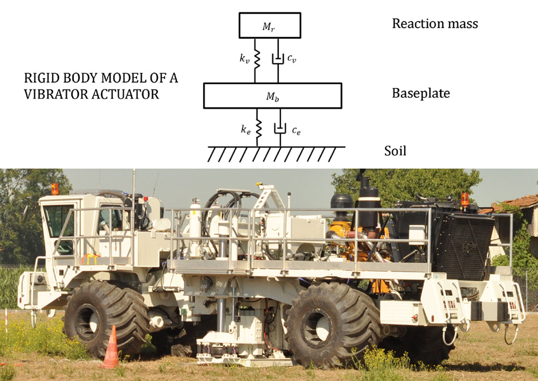
The usual truck-mounted, hydraulic seismic vibrator can be approximated to a harmonic oscillator (Sallas, 2010) (figure 1). The baseplate is held down with the weight of the truck to ensure coupling while the reaction mass is driven by the fluid passing through the piston cylinder. The accelerating reaction mass creates a counter-reaction force on the baseplate. At low frequencies, the baseplate and reaction mass are in phase, the plate being almost stationary while the mass moves. At resonance (around 20 to 40 Hz), the two have a 90 degrees phase lag and comparable accelerations. At high frequencies they have opposite phase and the baseplate acceleration dominates.

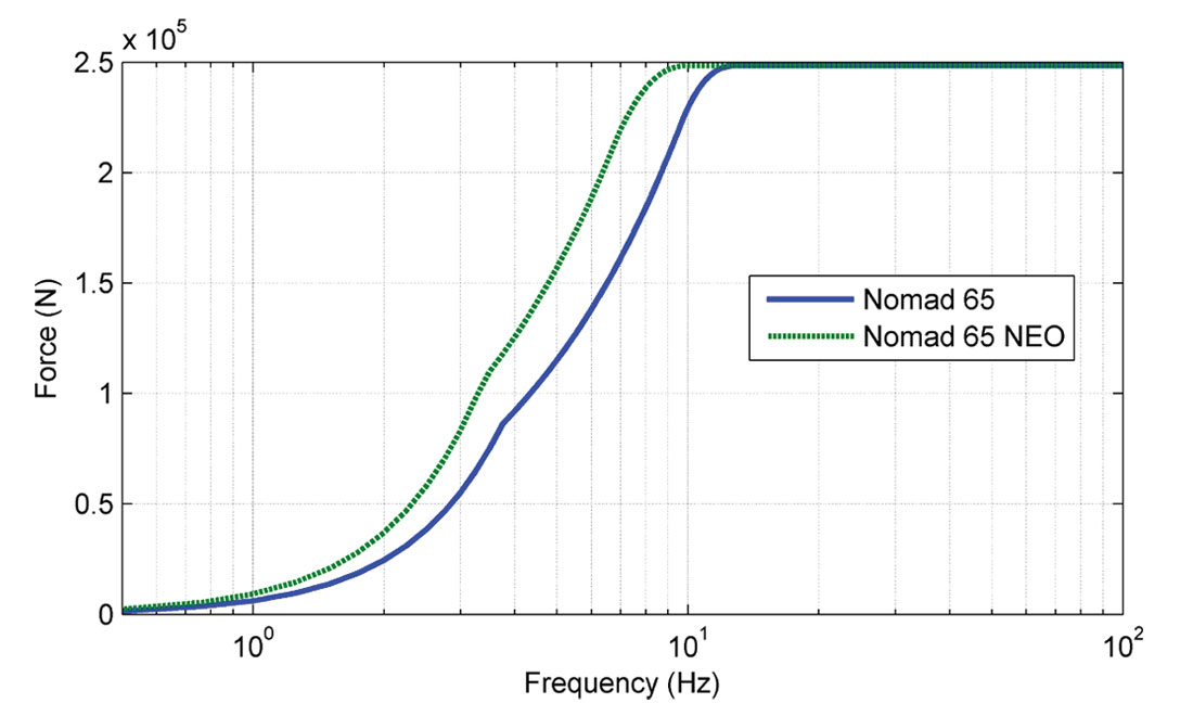
Below 5 Hz, the necessary travel of the mass may be larger than the stroke. This is intuitive: the longer the period, the longer the mass has to accelerate. The acceleration being the second derivative of the displacement with respect to time, the maximum output of the vibrator for a given stroke is proportional to the square of the frequency (Figure 2). Another limiting factor is the hydraulic pump flow required to maintain the circuit pressure when shaking low frequencies. The maximum force, taking into account the flow demand, is proportional to the frequency (Figure 2).

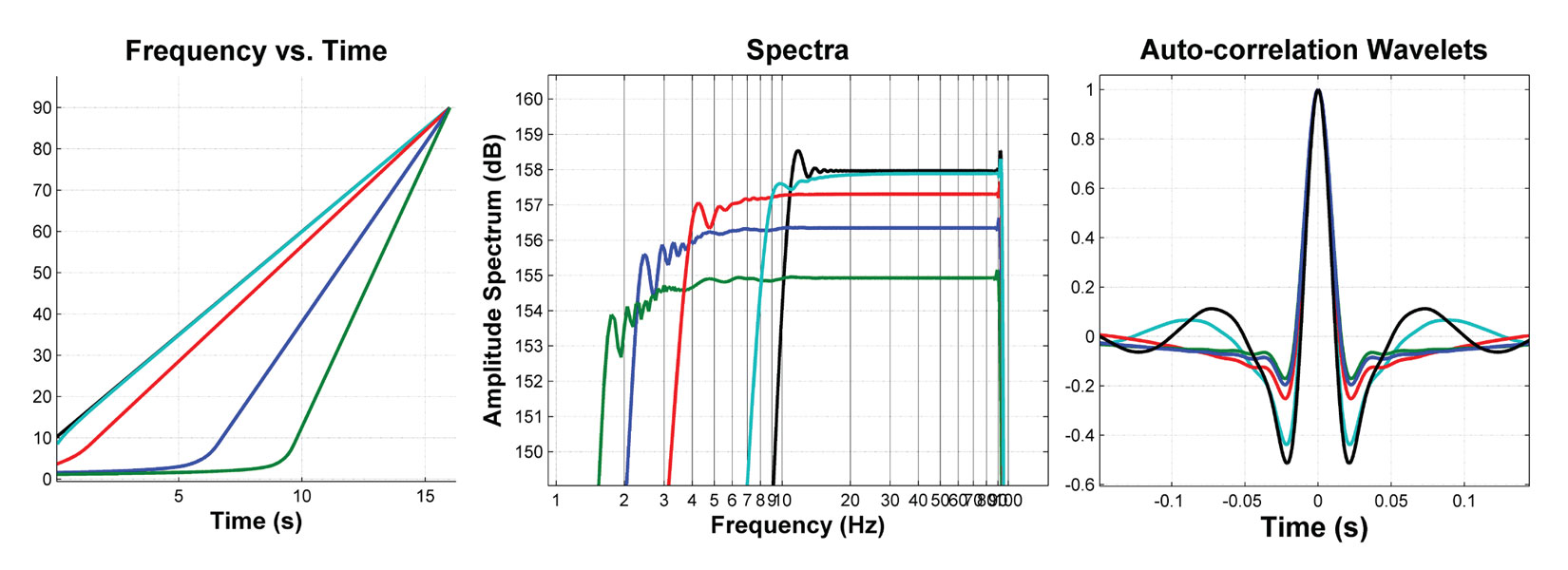
Once the maximum force output has been derived from the mechanical specifications of the vibrator, any spectrum shape can be achieved by modulating the sweep rate (Baeten et al. 2010, Meunier, 2012). The low force output at certain frequencies is compensated by spending more time, “dwelling” longer, than at full force frequencies. The result in the time-frequency domain is shown in Figure 3a for 16 seconds sweeps starting at 10, 8, 4, 2 and 1.5 Hz. Figure 3b shows amplitude spectra and Figure 3c the associated autocorrelation wavelets. Unsurprisingly the wavelets side-lobes are reduced as the bandwidth increases. For a given sweep length (ie. cost), the loss of energy versus the broadening of the bandwidth becomes significant below 3 Hz: -1.5 dB for a 2 Hz start and -3dB for 1.5 Hz. Put another way, to maintain the same energy over the shared bandwidth, we have to double the sweep length for a 1.5Hz start versus an 8 Hz start.

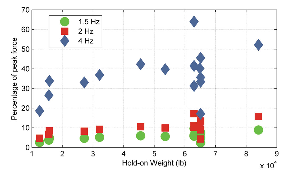
Another point to raise is the near absence of relationship between the weight of the vibrators and their low frequency output capability. Figure 4 shows the efficiency versus maximum force at 1.5, 2 and 4 Hz for 17 models of seismic vibrators. The maximum force is proportional to the hold-down weight, yet this does not prevent small vibrators from delivering low frequencies within their energy range. Several models of small seismic vibrators prove to be as efficient at generating low frequencies as larger vibrators (that is, relative to their peak force). Sensitive areas with shallow targets such as northern Alberta benefit from this technology just as much as deep target areas.

The sensors

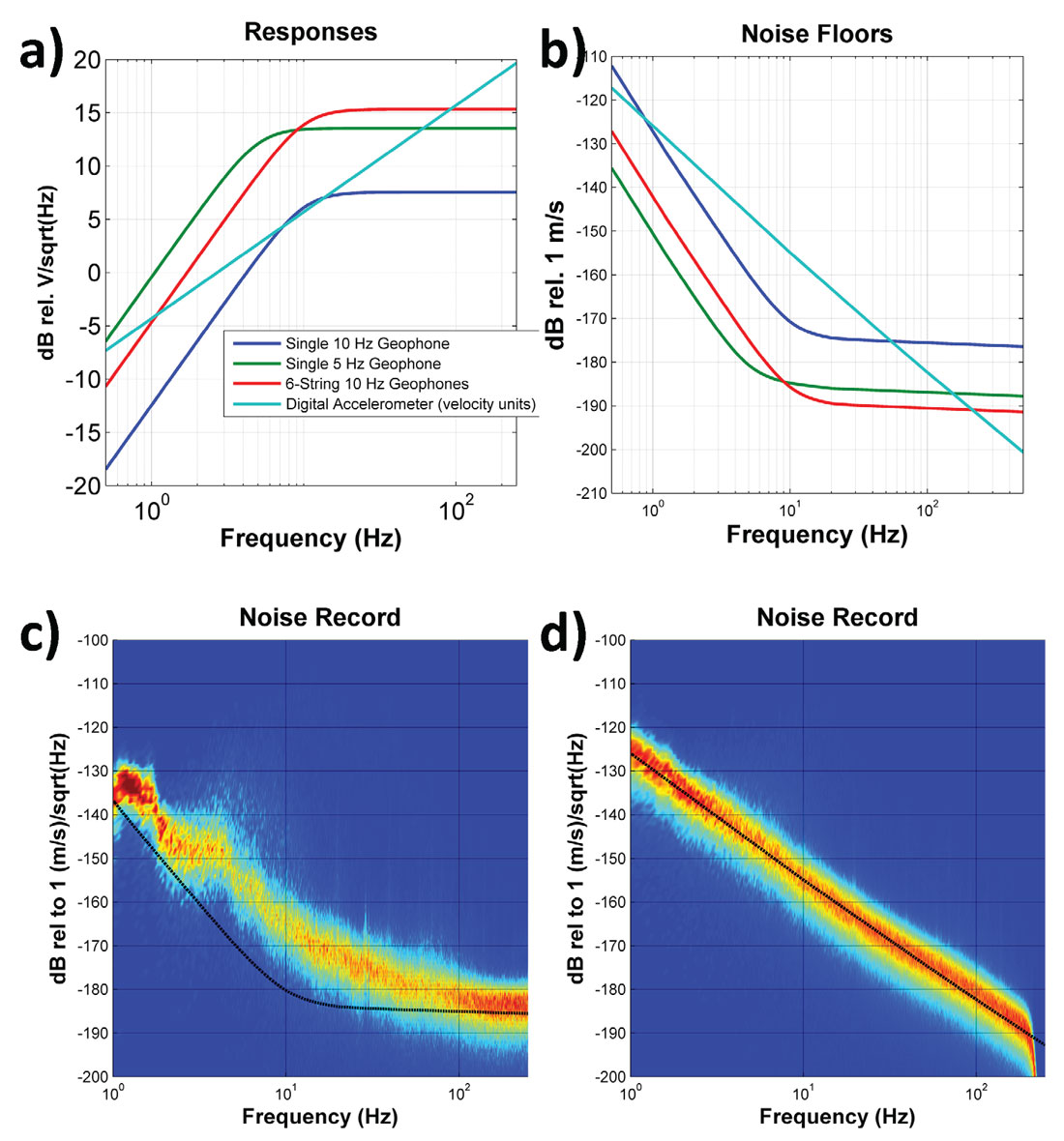
As with the hydraulic vibrator, the geophone may be modelled as a simple harmonic oscillator, where the sensor response is fully determined by the resonance frequency and damping. The response is scaled according to the sensitivity of the unit (Figure 5a). Connecting several units in series adds their individual sensitivities, at the expense of increased equivalent impedance which may result in induced noise pickup.

MEMS accelerometers have a flat response in the acceleration domain, which corresponds to a 6dB/octave straight line response in the velocity domain (Figure 5a).

To assess the lowest particle motion that can be detected on a non-summed recording, sensitivities have to be combined with the system noise (dominantly thermal, but also quantization) (Figure 5b). The optimal sensitivity is reached when the “ambient” noise, i.e. the noise recorded by the sensor, exceeds the thermal noise, as seen in (Figure 5c). Figure 5d shows a case where the system noise is prevalent. In this case system noise is the main adversary when seeking to retrieve the source signal, not the ambient noise, which means that more sensitive sensors would have been optimal. It is therefore advised that the sensor sensitivity choice should be determined according to the ambient noise level for maximum efficiency; sensitive sensors for quiet areas (Maxwell, 2011).

Sampling

Although this is an acquisition oriented paper, the authors feel a low frequency acquisition strategy has its full meaning only when associated with a processing strategy. Onshore broadband processing presents challenging aspects, which fall into 3 main categories: coherent noise, un-coherent noise and phase-fidelity.

Spatial sampling requirements are not as costly for low-frequencies. For example, at 5 Hz it takes 30 meter station interval to properly sample a slow 300 m/s ground roll, which helps the linear noise attenuation through velocity-filtering.

The pre-stack migration (pre-STM) modulates the signal to unorganized-noise ratio as a function of frequency. The Fresnel zone radius is inversely proportional to the square root of the frequency. If the migration is considered as a summation surface, a bigger zone of influence results in a larger signal summation order. The signal-to-noise ratio after migration is thus favourable for low-frequencies.

The phase-fidelity may be impacted by acquisition or processing steps. On the upside, statics do not prove as destructive for low frequencies as they can be for higher pitched waves, since a time difference represents a small phase lag. On the downside, a small phase-lag in the data may quickly result in large time-shifts. This area is not fully understood, and depends on the processing shop and its implementation of the seismic algorithms: window length selection, tapering and time-padding parameters can cause headaches. Phase-fidelity should therefore be controlled throughout the processing, by looking at the alignment of strong events on band-pass panels for example.

A demonstrated and easy ingredient for a successful broadband processing is to apply an inverse sensor response prior to deconvolution. In the absence of noise, the statistical estimation of the wavelet in the deconvolution should contain the sensor effect. A recent onshore example from North America proposed a match filter between measurements on standard and low frequency phones avoiding unstable inverse filters that provided satisfactory results (Chiu et al., 2013). In other examples from the Middle-East, the authors also advocate in favour of accounting for the sensor response as early as possible (Mahrooqi et al., 2011). In Denis et al. 2013, pre-STM images showed improved low frequency content after re-processing tests including the geophone response compensation.

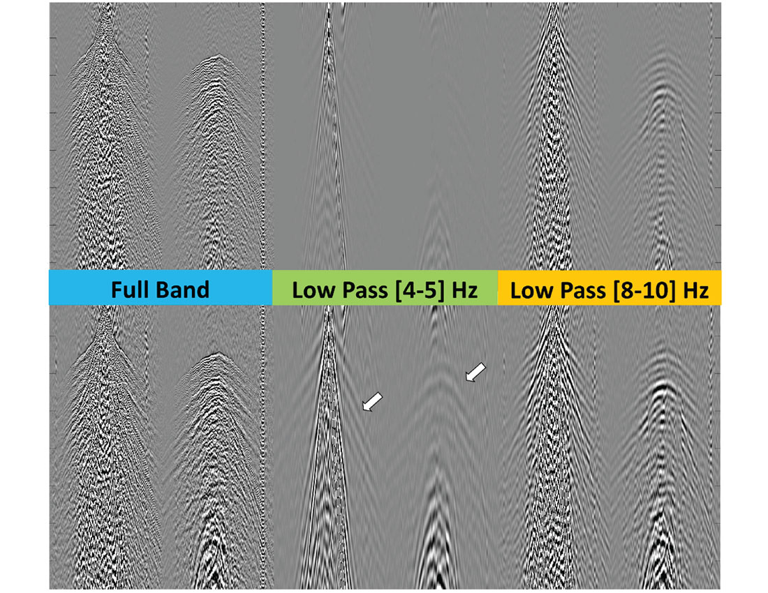
Figure 6 shows the difference before and after application of an inverse geophone filter on shot gathers. Before application, P-wave energy is barely visible on the shot gathers below 5 Hz. After application, linear refracted energy is clearly visible. The phase shift of low frequencies due to the sensor response results in a scalable time shift, visible on low-pass filtered sections. Early application of those corrections is the first step to ensure fidelity of low frequency signal during processing, such as linear noise attenuation, deconvolution and residual statics.

Case studies

This section shows some illustrations of low-dwell acquisition, mainly in North America, outlining some characteristics of pre-stack data.

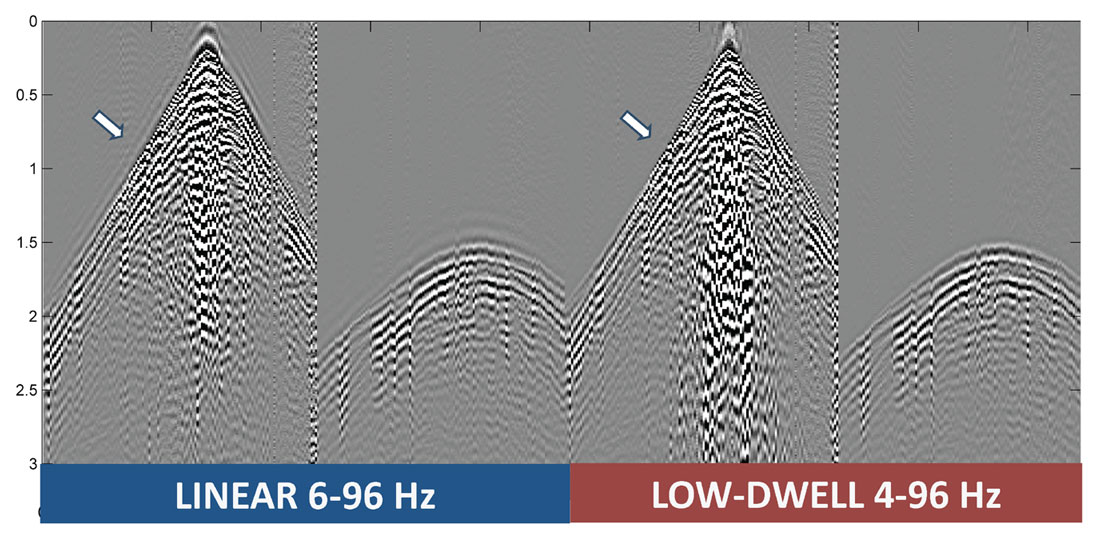
Figure 7 shows field gathers acquired with 4 linear, 10 seconds 6-96 Hz sweeps versus the same parameters with a 4 Hz start. The first-breaks exhibit the same spiky, reduced side-lobe characteristic as the theoretical wavelet. The surface-wave cone is stronger on the low-start sweep, the gathers after high-pass filtering are similar. Should the linear noise attenuation fail, a windowed high-pass filter targeting the noise cone can always be a drastic, last resort option.

Figures 8 and 9 show shot gathers acquired in Alberta and Alaska, split in several band-pass filters. The vibrator array contained three 270,000 N peak force units in both cases. On the receiver side, strings of 10 Hz geophones were laid out. The gather displayed used a sweep that began from a 4 Hz corner frequency. On the low-pass panels low frequency source generated ground roll dominates, yet refracted and reflected body waves are visible; evidence that reflected energy is present.

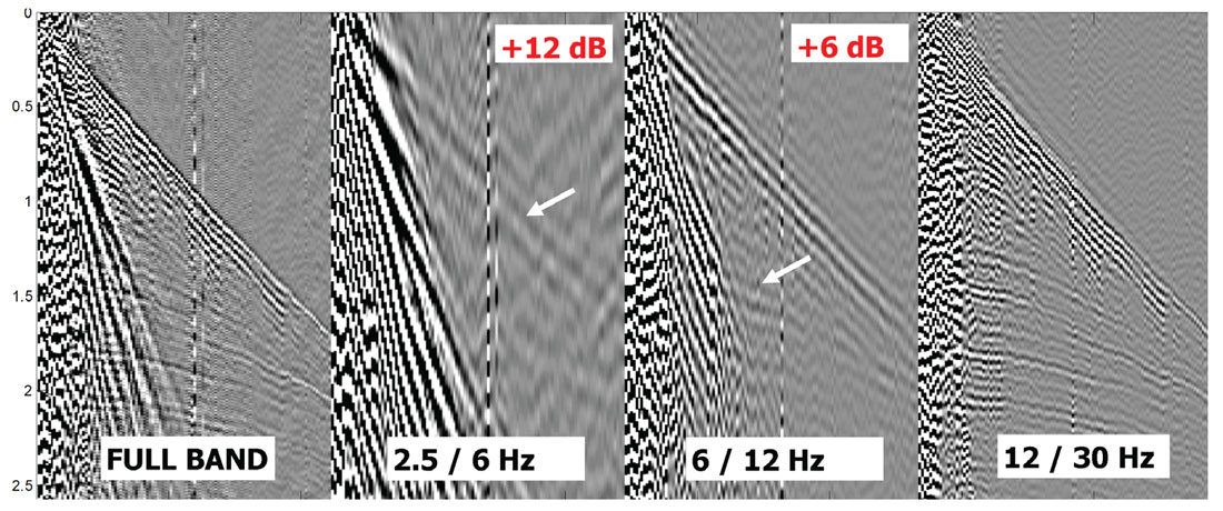
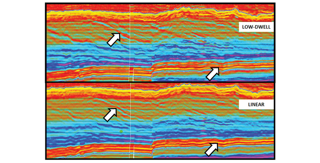
Figure 10 shows the result of a post-stack inversion on the Alaskan dataset with and without the 4 to 8 Hz frequency band. The full-band inversion shows improved resolution, higher contrast and better layer separation using the added low frequency content.

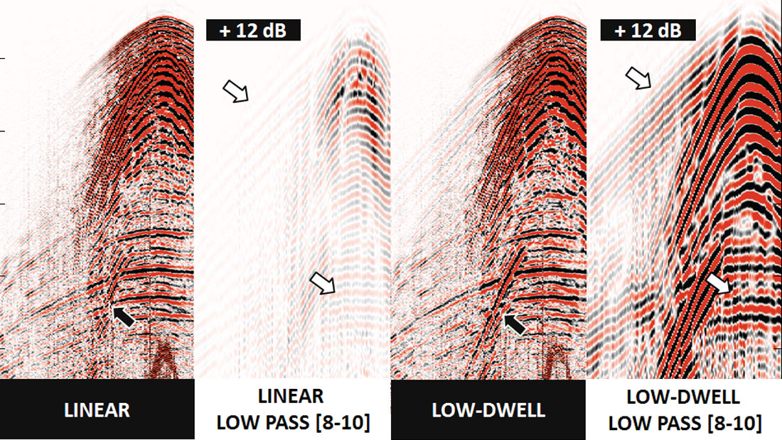
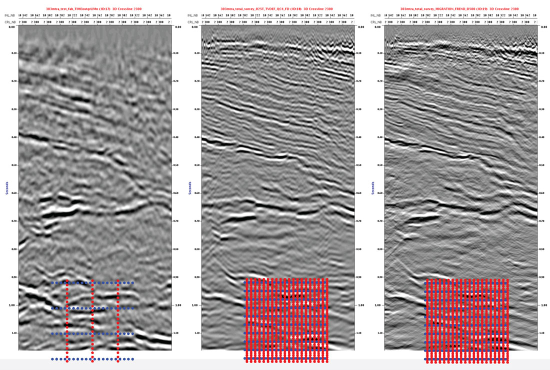
Figure 11 shows a shallow imaging example from South-Africa. A sparse, legacy dataset post-STM of 10-90 Hz is compared to filtered and full versions of a dense recent acquisition. On the recent acquisition the full-band exhibits a sharp and contrasted character the filtered version doesn’t. But the huge difference between legacy and recent survey comes from a source density increased more than ten-fold, using single sources and simultaneous shooting. This may be a reminder that however important bandwidth extension may be, it is not and will not be a substitute for the main driver of quality seismic: proper spatial sampling of the wavefield.

Conclusions

Onshore, it is possible to generate low frequencies by modulating the sweep rate according to the maximum output of the vibrator as a function of frequency. On the receiver side, standard geophones may be used as long as the sensor response is accounted for in the processing, while accelerometers have a flat response in acceleration domain.

Affordable broadening of the bandwidth towards the low frequencies (down to 2.5/3Hz) with conventional equipment and methodology has been demonstrated. Going lower has to be matched by increased source effort. In both scenarios, acquisition has to be followed by an adapted processing flow including early sensor response deconvolution and phase quality controls at several steps.

Broadband acquisition followed by broadband processing will lead to the perks of a spikier wavelet, deeper penetration and easier low frequency model recovery from seismic amplitudes when inverting for Earth properties.

Acknowledgements

The authors thank AngloGold Ashanti, Talisman Energy and the CGG Multi-Client and New Ventures group for allowing us to present their data.

Sincere thanks to Michel Denis of CGG for granting his permission to reproduce figure 12 from Denis, 2013.