Introduction
Interpretation of subsurface geology is greatly enhanced by 3-D seismic data, and this accounts for its ubiquity in today’s search for hydrocarbons. Seismic interpretation has two fundamental disciplines at its core: seismic geomorphology and seismic stratigraphy. Plan views allow the interpreter to apply principles of geomorphology, based on analogies with modern sedimentary systems, to interpret depositional environments and even predict facies distributions. On the other hand, section views require stratigraphic interpretation and give insight into stratal architecture and the temporal development of the depositional system. Both approaches give insight into the geological processes that formed the hydrocarbon play (eg Posamentier 2003).
This paper explores some of the techniques available today to take this insight to deeper levels than ever. The widespread availability of powerful computers and high performance graphics have opened new doors to the seismic interpreter, allowing him or her to test and tweak parameters to fine-tune an attribute, and to make unique and compelling displays to help them tell their story. Many of these techniques are especially potent if time is short: a quick, simple interpretation of a couple of easily-interpreted horizons is enough input to guide a rich assemblage of sophisticated algorithms through the dataset, revealing hidden patterns and subtle features in a matter of minutes. If more time is available, techniques such as 2-D seismic modelling can shed light on difficult interpretation problems and give m o re confidence that he or she is indeed interpreting geological features and not geophysical artefacts. We present examples of both of these approaches in this paper.
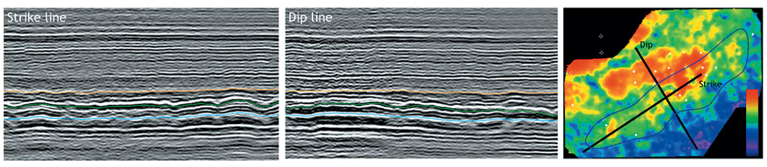
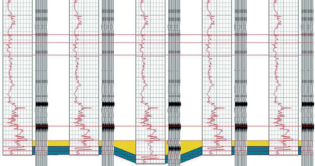
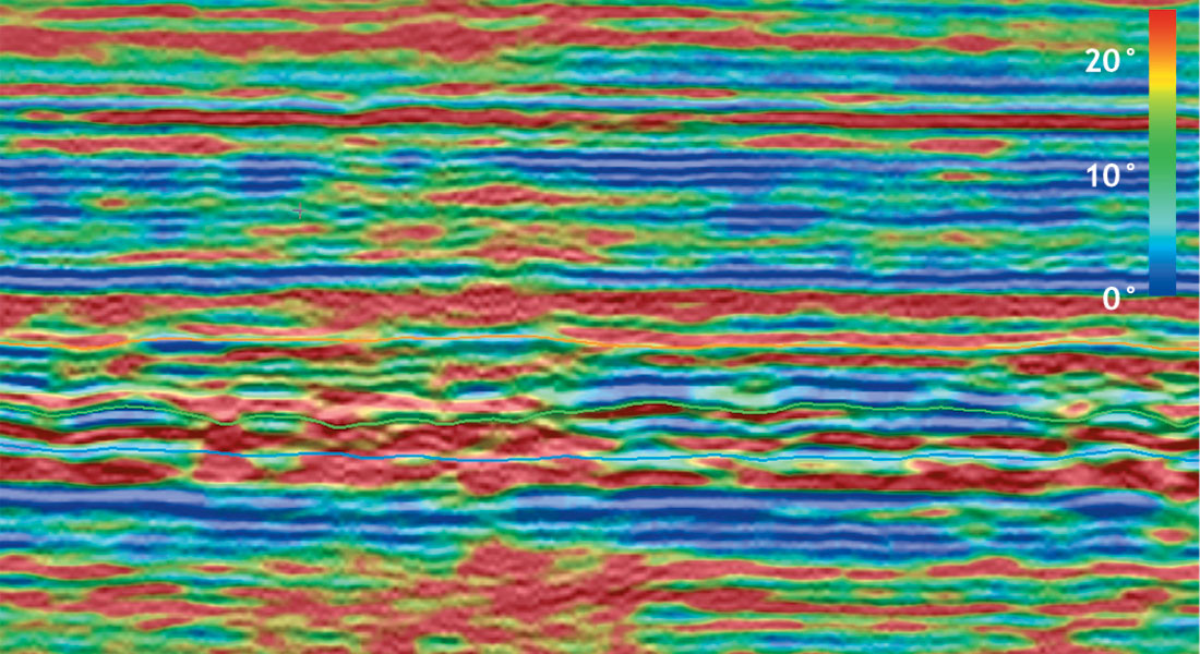
The example seismic dataset, shown in Figure 1, is a migrated full-stack, filtered, 16-bit floating-point amplitude volume from a producing oilfield in western Canada. We interpreted three horizons with sparse seed lines and an autopicking tool; all three horizons were finished in under an hour. The horizons were interpolated and smoothed and are used for building a velocity model for depth conversions, and for guiding the attribute extraction algorithms along structure. The reservoir interval is interpreted as a tidal sandridge complex deposited during a lowstand and transgression in the early part of the Mississippian. Offshore shales are unconformably overlain by heterolithic lower- and then sandy upper-shoreface sandbodies, which are subsequently partially reworked and redeposited as tidal sand-ridges during a period of transgression. These sands are then conformably overlain by the ensuing highstand shales. The sand ridges are around 20–40 km long, 3–7 km wide, and 20–30 m thick, and these are the subject of our investigation.
Seismic Stratigraphy
Modelling
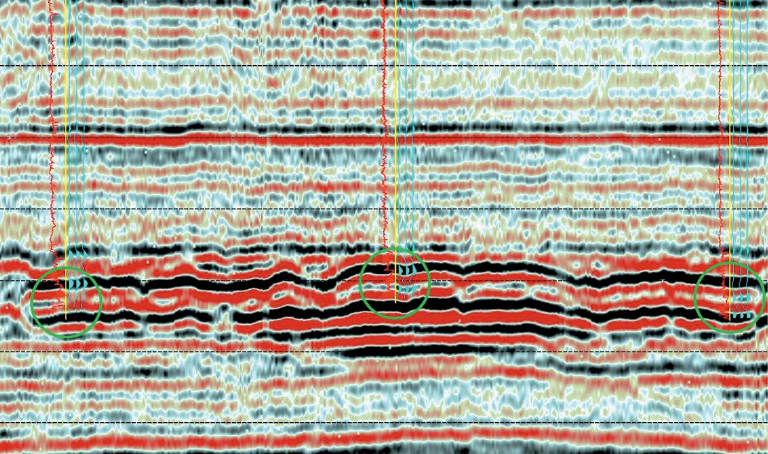
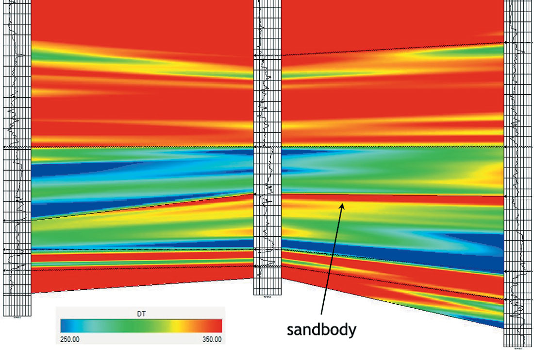
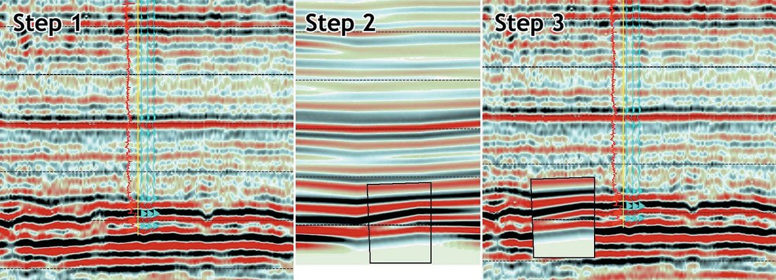
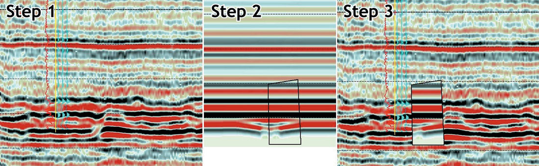
Seismic volumes are complex volumes of reflections, interference and tuning effects. It can be difficult to know what to expect a given sandbody or stratigraphic geometry to look like in the seismic. Seismic modelling can give the interpreter this insight, and allow him or her to try multiple iterations in order to best match a known response. Stratigraphic interpretations can then be made in areas where there is little or no well control.
A workflow for seismic modelling to illuminate stratigraphic relationships is illustrated in Figures 2–6.
Volume seismic attributes
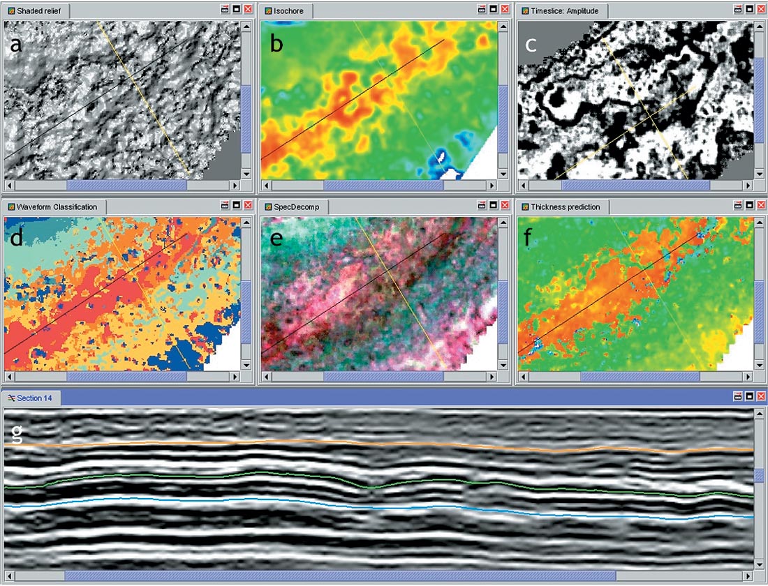
Attributes drawn from a group of seismic traces in a 3-D volume are capable of representing complex three-dimensional reflection characteristics and relationships. For example, it is possible to generate a volume representing the amount of dip or degree of parallelism displayed by the reflectors in the seismic. These are calculated directly fro m the seismic traces, with no interpretive input (though the quality of the results are improved by the use of a three-dimensional velocity model, which normally would incorporate some surface interpretations to guide the velocity fields). Other such attributes quantify aspects of the reflectors such as continuity, hummockiness, divergence and azimuth. It is even possible to combine and reprocess these attributes to produce new ones, such as shaded relief images (Barnes 2003; see example in Figure 7a). These attributes all represent aspects of apparent palaeotopography, which can aid in geological interpretation. This is especially true when the results are combined with other images. Two effective ways of achieving this are semi-transparent overlays (Figure 8) and colour blending (Figure 9). As with all 3-D seismic datasets, using these visualization techniques in a 3-D space is more powerful still.
Waveform Classification
An important component of seismic stratigraphy is recognizing systematic variations in the character of a seismic reflector or set of reflectors. Such variations might reflect changes in stratal geometry or lithologic stacking patterns. This can be a powerful way of elucidating subsurface stratigraphy qualitatively and, when coupled with seismic modelling, quantitatively (eg Williamson 2003). An important feature of waveform classification is that wavelets are compared by shape, not by amplitude. This can mean that waveform classification is less affected by tuning effects and porosity variation, for example, than other types of seismic attribute.
There are two fundamental approaches to waveform classification: supervised and unsupervised. Supervised approaches require the interpreter to select a time-window (usually centred on a seismic horizon) and provide any number of reference waveforms (as an inline/crossline location). These are often chosen to be representative of distinct lithologies at nearby wells. For example, one might provide the location of an especially thickly-developed reservoir interval, a thinner reservoir interval, more heterolithic reservoir, a shaled-out reservoir section, and an eroded, unconformable section. These waveforms represent 5 discrete classes. Every trace in the seismic volume is then classified according to which of the reference waveforms it most closely resembles; there is also a ‘zeroth’ or reject class for traces which resemble none of the references. The result is a map of wavelet classes in which each class is represented by an integer.
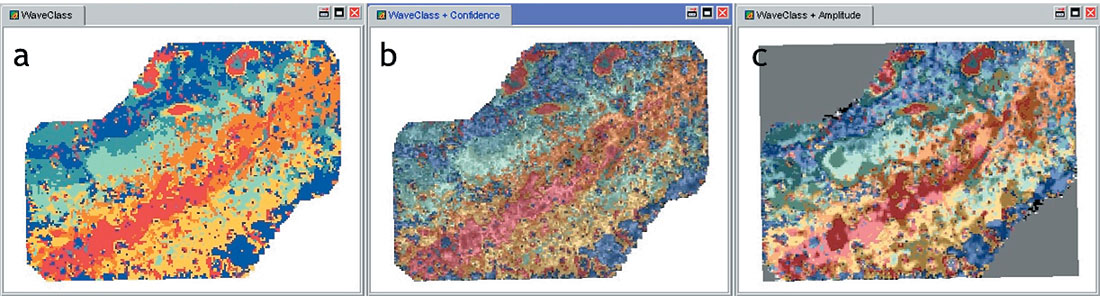
The second approach, supervised classification, automatically calculates a reference wavelet from the data before assigning classes. This is achieved by an iterative statistical analysis of a subset of the data, the results of which are then applied to the entire dataset. As before, the result is a map of waveform classes, such as those shown in Figure 10, with each class being re p resented by an integer. The classes are organized according to relative similarity, so class 1 more closely resembles class 2 than it does class 5. This approach is especially useful if there are no wells in the area of interest, or if the interpretation is in the early stages and no firm correlations with wells have yet been established.
Seismic Geomorphology
Spectral decomposition
Ordinary 3-D seismic data typically has a 60–80 Hz bandwidth, so it contains energy reflected from the subsurface at a wide range of frequencies, all of which are compounded in a typical seismic volume. In certain circumstances, especially subtle stratigraphic plays, it may be helpful to see the amplitude (or phase) of reflections at particular frequencies. These tuned amplitudes may tell the interpreter something about the physical spacing of the acoustic impedance contrasts in the image—in other words the bedding thicknesses (eg Partyka et al., 1999). There are also examples of mapping the attenuation of high-frequency signal by hydrocarbons, allowing their direct detection (eg Castagna et al., 2003). Spectral decomposition analysis allows the interpreter to quantify amplitude variation with frequency, and thereby gain insight into the distribution of different stratigraphic packages and/or hydrocarbons.
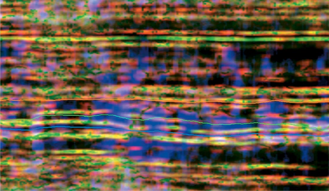
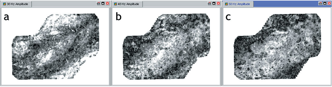
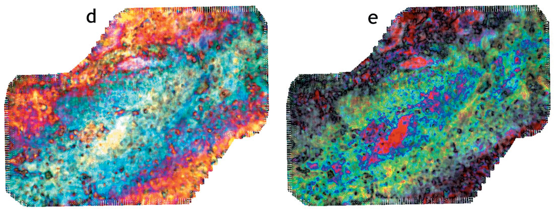
There are three key spectral decomposition workflows. The first is to process a discrete window a round a very smooth seismic horizon interpretation, transforming the amplitude or phase data into the frequency domain (in other words, a new volume results, with frequency represented by the z-direction; a typical volume might contain 100 slices, representing amplitude or phase at 1–100 Hz). Such a volume is called a ‘tuning cube’. There are two helpful ways of visualizing this dataset. The first is simply to animate through the volume, exactly as one would animate through timeslices. This yields images similar to those in Figure 11 a – 11c. The second visualization technique is to blend three timeslice images at a time, using the techniques illustrated in Figures 11d and 11e. Such blended images can provide an attractive and data-rich snapshot of very subtle reservoir characteristics. This workflow should help establish which features of the reservoir interval are brought out by which frequencies.
The second workflow is to leave the data in the time domain, but to process a series of time windows (a ‘running window’). Typically, a flattened seismic volume is used, with the same guiding horizon as a datum. The result is a flattened volume which is tuned to a specific frequency or set of frequencies, such as those established as useful or revealing in the tuning cube workflow. The reason for using a flattened volume is to give insight into the geological evolution of the interval. Animating through a tuned volume shows the same reservoir subtleties revealed in the first workflow, but now with the added dimension of geological time.
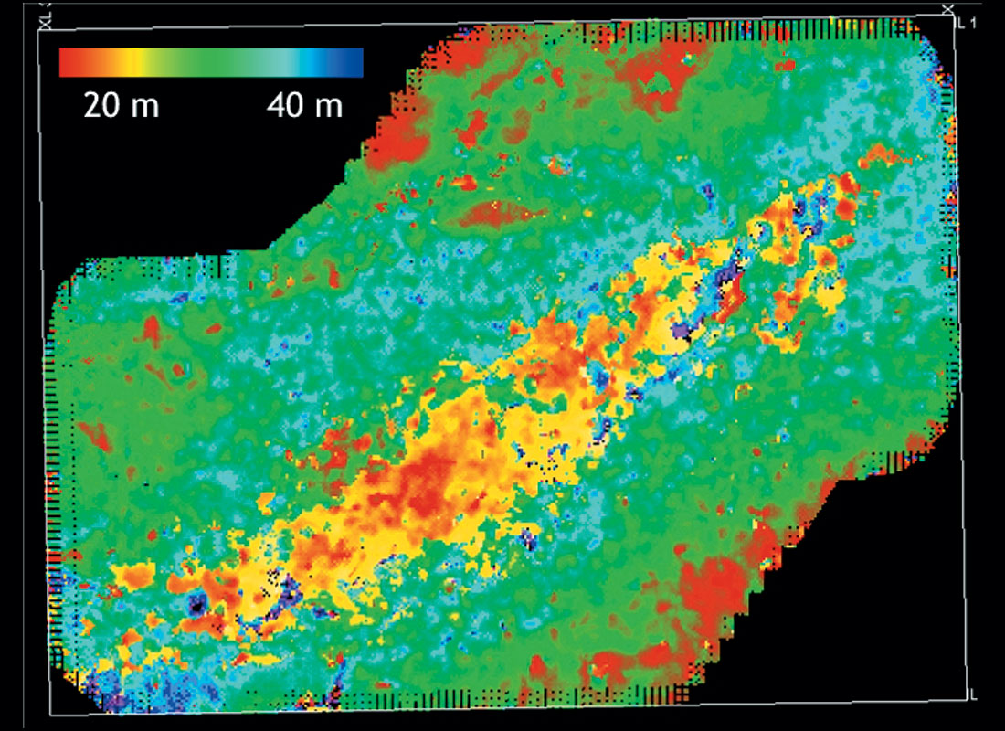
The third workflow gives a valuable quantitative estimation of bedding thickness in the analysis window, without the need for accurate seismic interpretation or phase concerns. Figure 12 shows an example of such a thickness estimation map, derived from the first spectral peak frequency attribute. This attribute is simply the frequency of the first peak in the amplitude spectrum . This is an important number, because it is exactly half the value of the spacing of the interference ‘notches’ in the spectrum. The notches are, in turn, spaced in inverse relation to bedding thickness in the analysis window. See Partyka et al. (1999) for a full explanation of the physics of this analysis. A simple horizon calculation can therefore transform the first spectral peak frequency attribute into time thickness, or, given the interval velocity of the zone, vertical thickness. Since this is an independent measure of bedding thickness, this workflow is potentially an important risk reduction tool for the explorationist. The approach is especially powerful when coupled with synthetic modelling and/or crossplotting the predicted thicknesses with actual vertical thicknesses as measured in offset wells.
These workflows, well-proven by several years of application in the industry, can give valuable insight into the internal organization of the reservoir interval. We have found the images and animations particularly effective communication tools, particularly in plays with strong stratigraphic components such as channel sands and deep marine gravity deposits.
Instantaneous seismic attributes
There is an almost bewildering number of instantaneous seismic attributes, each of which describes some aspect of a single trace at a single time or time-window. Examples include simple attributes such as phase or reflection strength, and more sophisticated interval statistics such as number of zero-crossings or total time thickness above a given amplitude. Maps of these attributes can often be interpreted geologically, with some features drawn out by particular examples. The ability to view many maps simultaneously, with a range of different colourbars and zoom-levels, can be a significant aid to interpretation. An example is shown in Figure 7, in which six maps are compared side-by-side. This allows the interpreter to quickly spot correlations or discrepancies between attributes which may have stratigraphic explanations. Opacity overlays and blended images may also help with interpretation, as previously illustrated in Figures 7–11.
Another technique for multi-attribute analysis, and for correlating seismic attributes with reservoir properties or with each other, is crossplotting. An in-depth review of this technique is beyond the scope of this paper, but many examples can be found in the literature. Establishing a relationship with a reservoir property is especially useful, since it allows the interpreter to model and predict the property directly from the seismic, with a known and quantifiable level of certainty. This makes the analysis of exploration risk considerably easier.
The Power of Volume Interpretation
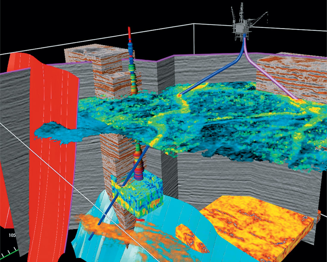
While this paper is focused on two dimensional views of the seismic data, volume visualization and interpretation is now well-established as an interpretation discipline. A 3-D seismic volume has not been truly interpreted until it has been volume interpreted (Figure 13). Despite this, it remains curiously ‘niche’ or somehow ‘advanced’ in the Canadian geoscience community (but that’s another story!). Two basic aspects of volume interpretation make it an important tool for the stratigraphic investigator: rapid volume interpretation and surface visualization.
The ability to instantaneously track an amplitude anomaly or apparent pinchout, and see the results in three dimensions alongside key reference data such as well logs and fault interpretations transforms the slow, methodical, line-by-line interpretation task into a dynamic and much more creative process. Hunches can be instantly verified, or disproven, and leads can be rapidly generated and investigated. More powerful still is the ability to bring multiple seismic attributes to bear simultaneously on a problem. Some great examples of applying these techniques to stratigraphic problems are shown in Meyer et al. (2001) and Alexander et al. (2001).
Surface visualization is an important tool for seismic geomorphological studies (for example, see Posamentier 2003). Viewing angle, lighting direction, colour, texture, and vertical exaggeration can be instantly adjusted to bring out the particular features of a seismic horizon. Misties and other anomalies can be seen and corrected. Attributes can be overlain on structural surfaces and visual correlations made. The interpreter can learn more in minutes of playing in 3-D than in days of looking at maps.
Conclusions
A very rich set of tools is available to the seismic interpreter for gaining insight into stratigraphy. Which tools one chooses to apply depend on the play type being investigated, the amount of time available for analysis, the stage in the interpretation process, the quality and nature of the available data, and the preferences , experience and intuition of the individual. There is no formula for the ‘right’ attribute for a given situation. In fact, our own approach is to build as many models, look at as many attributes, and try as many parameters as time allows. Time saved by automatic surface interpretation and volume interpretation can be put to good use by applying the available tools, letting the data itself offer up the answers. This seems like a better use of time, and technology, than the frustrating process of line-by-line interpretation of difficult surfaces, the results of which are always risky and uncertain.

Acknowledgements
We would like to acknowledge Landmark Graphics for permission to publish this paper. PowerView, PowerCalculator, SpecDecomp, PostStack, GeoProbe, Wellbore Planner, SeisVision, LogM and GESXplorer are trademarks of Landmark Graphics.


Join the Conversation
Interested in starting, or contributing to a conversation about an article or issue of the RECORDER? Join our CSEG LinkedIn Group.
Share This Article