A Reservoir Characterization Strategy for the Flemish Pass Basin, Offshore Newfoundland and Labrador

In frontier deep water exploration settings such as the Flemish Pass offshore Newfoundland and Labrador, wells are uncommon and are often separated by tens of kilometres or more. Given the scarcity of well data, well-to-seismic calibrations must be extrapolated over large distances. Seismic interpretation and analysis drives the understanding of components of the petroleum system, prospect evaluation and the selection of drilling locations.

The use of seismic data in the detection of reservoir presence and in the discrimination of reservoir quality and fluid-fill are challenging tasks that are of interest in this study. In this frontier setting, amplitude versus offset (AVO) reflectivity and inversion methods are critical to this endeavour. A review of these methods is not within the scope of this work; an excellent summary of the state-of-the-art of reflectivity and inversion methods is provided by Russell (2014).

In this study, three exploration wells drilled in the Flemish Pass Basin are examined. Lithology fluid prediction (LFP) logs have been calculated for each well, and synthetic seismic panels and crossplots have been generated. The goal is to determine the seismic attributes, whether reflectivity- or impedance-based, that are most appropriate to understand variations in lithology, reservoir quality and fluid content in this geologic setting. This will inform a general strategy for reservoir characterization from seismic data in the Flemish Pass Basin.

Regional Setting and Wells of Interest

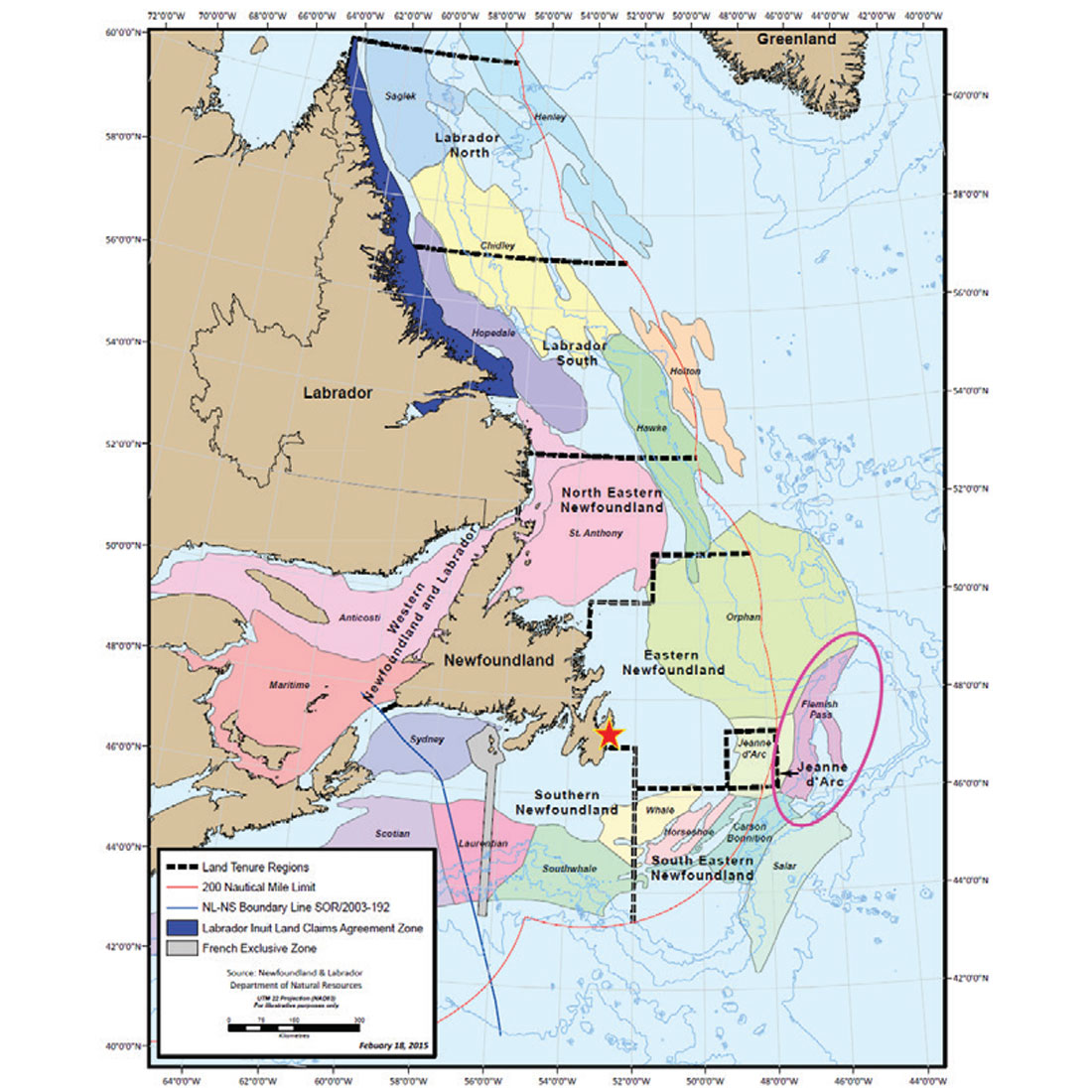
The Flemish Pass Basin is located in the North Atlantic Ocean, roughly 400 km east of St. John’s, Newfoundland and Labrador as shown in Figure 1 (C-NLOPB, 2015a). The basin is adjacent to the producing Jeanne d’Arc Basin and frontier Orphan Basin. As of year-end 2015, Statoil is the operating partner for five exploration licences and two significant discovery licences in the Flemish Pass Basin. Additionally, in November 2015, the Canada-Newfoundland and Labrador Offshore Petroleum Board (C-NLOPB) announced the results of a call for bids, and indicted that Statoil was the successful bidder as operator for five new exploration licences, and as a non-operating partner in an additional exploration licence (C-NLOPB, 2015b). These licences are expected to be awarded in early 2016.

The first exploration well was drilled in the Flemish Pass in 1985, and none followed for nearly two decades. Statoil entered a partnership to explore the basin in 1998. In 2003, oil was discovered in the partner-operated Mizzen L-11 well. In 2009, Statoil as operator drilled the Mizzen O-16 oil discovery, and followed in 2013 with oil discoveries at Harpoon O-85 and Bay du Nord C-78. Oil discoveries are in Upper Jurassic sandstones deposited in a fluvial-estuarine environment. For each well, multiple sands of varying quality and fluid-fill have been encountered. Additional delineation and exploration has followed since 2013, and as of year-end 2015, 13 wells or sidetracks have been drilled in the basin in a licenced area covering approximately 8500 square kilometres.

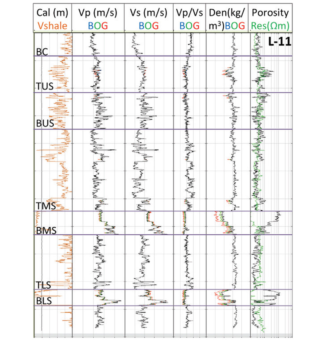
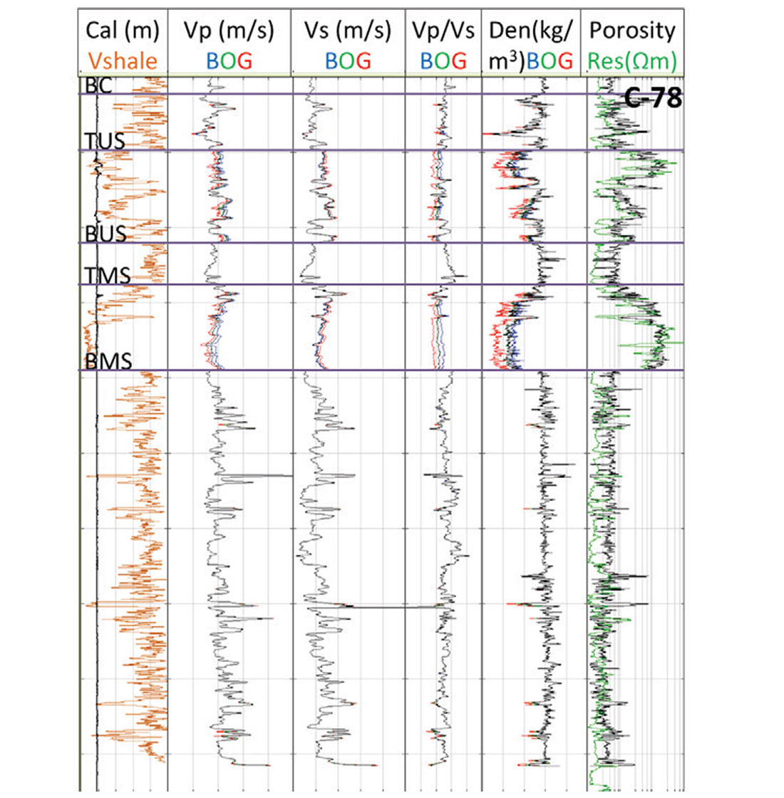
Figures 2-4 respectively show well logs for Mizzen L-11, Mizzen O-16, and Bay du Nord C-78. Only the Upper Jurassic interval is shown for each well, with the uppermost top marking the Base Cretaceous (or Top Jurassic). The main Upper Jurassic sands when present are designated as upper, middle, and lower in each well. These names represent approximate age correlations, but sand bodies may have been deposited in different depositional fairways and experienced different diagenetic alteration. For each well, the Vp, Vs, Vp/Vs, and density logs are shown as recorded and for brine, oil, and gas fluid substitution scenarios. Gassmann (1951) methods have been used for fluid substitution. For consistency with the discovery cases, L-11 and C-78 oil substitutions use light API oil, and O-16 uses medium API oil. For all logs, values increase to the right.

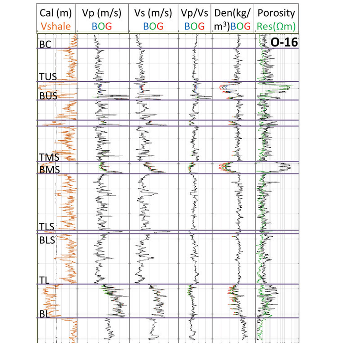
In L-11 (Figure 2), the upper sand is poor quality with a thin net interval, while the middle and lower sands have thicker net intervals, are clean at the top and cemented with calcite at the base. The fluid-substituted logs show the most variation in the top portions of both the middle and lower sands. In O-16 (Figure 3), the upper and middle sands are of most interest, with the upper sand clean and high porosity near the top and cemented with lower net-to-gross near the base. The middle sand is clean with high porosity, with a cement streak at the base. The effect of fluid substitution is clear in both of these sands. For C-78 shown in Figure 4, the upper sand is thick with moderate net-to-gross while the middle is thick with a gradational top and clean base. These sands lack cemented zones and strong fluid substitution effects are evident.

Lithology and Fluid Discrimination from Logs

Reflectivity Methods

Firstly, reflectivity-based methods will be considered following the concepts outlined in Rutherford and Williams (1989) and Castagna and Swann (1997). As shown in Figures 5-7, synthetic seismic gathers have been created for each well for the fluid substituted brine, oil, and gas cases with angles up to 50 degrees displayed. Amplitude vs. offset curves are considered for selected zones and intercept and gradient traces have been calculated for the interval examined. In some cases (as noted below) the critical angle is reached prior to 50 degrees, so in all cases the intercept and gradient tracks are calculated from 0-40 degrees. For all synthetic tracks, a red trough represents a decrease in impedance while a blue peak in an increase. The “N” represents the near trace, “F” the far trace, “FS” the full stack trace. The bold red and blue lines on the synthetic traces show the positions from which the amplitudes were taken for display in the AVO panels.

Figure 5 shows the synthetic gathers for C-78. First fluid prediction for the middle sand will be considered. A moderate amplitude peak marks the top of the gross interval, and the high porosity zone below the gradational top is a strong trough for all fluid fill models. The amplitude curves suggest that the top porosity response is a Class IV (Castagna and Swann, 1997; Young and LoPiccolo, 2003) for all fluid scenarios. This is confirmed by the intercept and gradient tracks that show a strong negative intercept and a weak positive gradient. The fluid effect is observable in the intercept, as the trough amplitudes progressively increase from brine to oil to gas models, and to a lesser extent in the gradient with gas fill having the highest positive value. The base of this sand is a peak, with intercept values strongly correlated to fluid (strongest values for gas, decreasing for oil and brine), and a weak positive gradient. Thus for the top and base of the middle sand where no cement is observed, fluid effects are manifested in the intercept, and the gradient values are low.

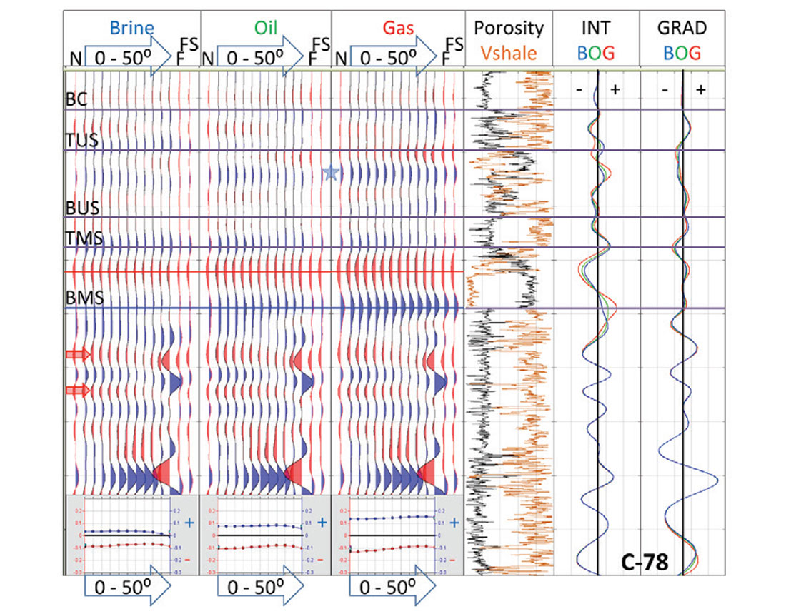
For the upper sand at C-78, no AVO curves are shown, but the intercept and gradient panels are illustrative. For the top upper sand pick, a fluid effect is observable in the intercept, as intercept values cross from positive to negative as fluid fill is changed from brine to oil to gas. The gradient is negative for each scenario (most negative value for gas), suggesting that the top sand is a Class II trough anomaly in the gas case and a Class II peak anomaly in the brine and oil cases (Rutherford and Williams, 1989). As might be expected for Class II responses, examination of the synthetic panels shows that the event at the top of this sand has extremely low amplitude, except at far offsets in the gas case. Given the weak amplitudes, it is possible that this event would never be interpreted on a real 3D seismic full stack volume; perhaps this porous sand interval would not be identified pre-drill. Similarly, there is no pickable event at the base sand, although there is a peak at the base of porosity in the upper sand (marked with a blue star) that is most prominent on the gas-substituted synthetic.

Lithology interpretation from reflectivity data is a challenge at C-78. Note the troughs below the middle sand annotated with red arrows in Figure 5. Each has a strong negative intercept and would likely be observable (and pickable) on a full stack, even if the gathers were muted beyond about 40 degrees to avoid post critical reflections. Each trough also has a positive gradient (below 40 degrees), making them Class IV to Class V (Young and LoPiccolo, 2003). This behaviour is similar to that of the middle sand, or as will be discussed next, is similar to the behaviour of cemented sands observed in L-11 and O-16. The Vshale and porosity logs show that these events are very shaley and very low porosity; they are not reservoir sands. Thus intercept-gradient interpretation of lithology is ambiguous.

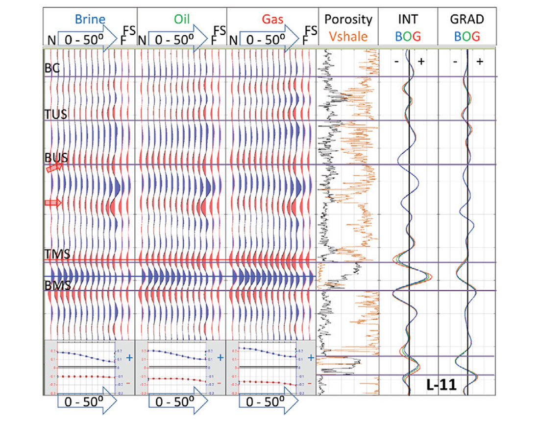
Synthetic gathers for L-11 are displayed in Figure 6. The middle sand is similar to the middle sand observed in C-78 (clean, high net-to-gross) with the exception that the base of the sand in L-11 is cemented, while the base of the sand in C-78 maintains high porosity. The average porosity of this sand is also higher in C-78 than in L-11. At L-11, the top of porosity for the middle sand is a strong trough for all fluid fills, with intercept value most negative for gas, least negative for brine. The gradient is near zero, suggesting that the top porosity is a Class IV and perhaps trending to a Class III (Rutherford and Williams, 1989) if farthest offsets are considered. The gradient displays no fluid dependency. The top of the cemented zone is a strong peak that weakens with offset. It is a Class I (Rutherford and Williams, 1989), with intercept suggestive of fluid fill (gas-fill giving the brightest intercept). The base of the sandy interval is a trough with a strong positive gradient, making it a Class V (Young and LoPiccolo, 2003). There is no fluid effect at the base sand due to reduced porosity from calcite cementation.

At first glance, the interval below the base upper sand (troughs annotated with red arrows on Figure 6) is similar to the middle sand response. Strong troughs with weak gradients are separated by a strong peak with a weak gradient (limiting angles to about 40 degrees in each case). This might lead to an interpretation of a Class IV sand with a cement streak, but the porosity and Vshale curves suggest otherwise. Like C-78, it seems that for L-11 lithology estimation is a challenge, but fluid interpretation is possible.

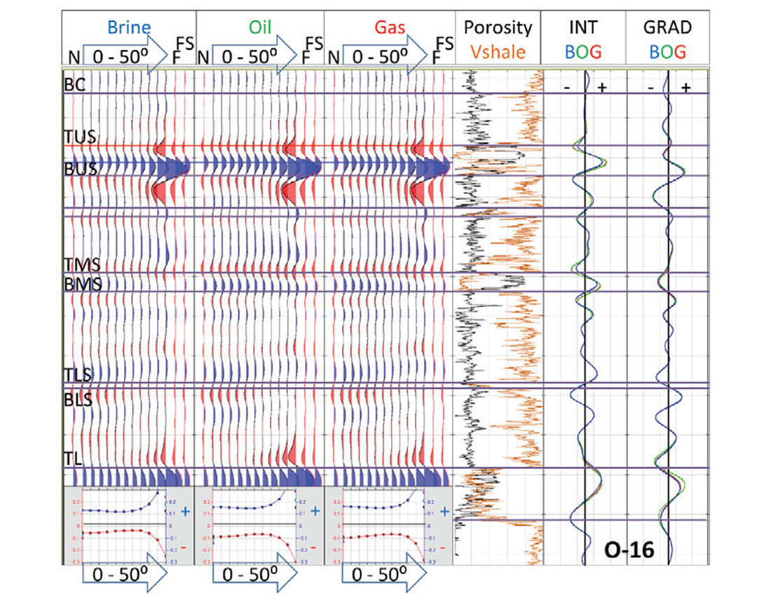
Both fluid and lithology interpretations are a challenge at O-16 (shown in Figure 7), perhaps due to thin beds and lower-net-to-gross zones. The upper sand has moderate net-to-gross and cement streaks. The reflection from the top sand is a trough with intercept variation according to fluid fill and a low positive gradient until the critical angle is reached around 40 degrees. It is a Class IV. The top of the cemented zone is a strong peak with a weak negative gradient (making it a Class I) until the critical angle is reached, also around 40 degrees. The base of the sand has a similar response as the top. The middle sand has a Class IV anomaly at the top and a Class I at the cemented base. Like the upper sand, the gas and oil substituted intercepts overlap. For the rest of the interval shown above the limestone (not examined), there are no strong reflections that would likely be interpreted on a full stack.

A Class II AVO anomaly was inferred for the upper sand at C-78, and a Class III for the middle sand at L-11 (if far offsets are included). A Class IV AVO anomaly has been observed for sandstones in each well, including the high porosity middle sands in C-78 and L-11 at angles below 40 degrees. Conversely, AVO Class IV was also interpreted for shaley, non-reservoir zones in C-78 and L-11. These Class IV observations lead to ambiguity in lithology interpretation. It is known that a Class IV could represent the top of a low impedance sand (Castagna and Swann, 1997, Foster et al., 2010), but this this might be considered an atypical response. In general, we might expect the top reflections for hydrocarbon bearing sands to be Class II or III AVO anomalies (Rutherford and Williams, 1989).

Nevertheless, the appearance of the Class IV reservoir sand is consistent with observations in the adjacent Jeanne d’Arc Basin. Royle et al. (2004) report several classes of AVO anomalies for a variety of oil API values in Cretaceous-aged sands, including Class IV for regions of poor reservoir quality. In contrast to this, Statoil workers Løseth et al. (2011) suggest that the top of a hydrocarbon source rock is often a Class IV AVO anomaly. Similarly, Avseth and Carcione (2015) cite a Norwegian Sea example where a Jurassic sandstone was interpreted from 3D seismic AVO anomalies, yet turned out to be the Draupne Formation source rock.

If reflectivity analysis of seismic data with no or limited well control is the only tool for reservoir characterization, then interpretations will be highly uncertain. One would be encouraged by the presence of troughs on the full stack or intercept volumes and particularly Class II or III AVO anomalies. However, one might be discouraged by the appearance of Class IV and thus never drill the best reservoir section at C-78. Fortunately, the cemented streaks within otherwise clean sandstones are generally peaks on the full stack and intercept with Class I AVO, making them easy to distinguish. If sandstone reservoir presence was interpreted, then fluids could be inferred as generally the intercept becomes more negative as fluid is substituted from brine to oil to gas.

Impedance Methods

Next, impedance-based or seismic inversion-based methods are considered. The primary logs analyzed are lambda-rho and mu-rho (Goodway et al., 1997) rather than P- and S-impedances. Goodway (2001) illustrates that lambda-rho and mu-rho are in general more sensitive to key petrophysical parameters such as porosity, fluid saturation and lithology than are P-impedance, S-impedance, Poisson’s ratio and Vp/Vs ratio. Similarly, separations in crossplots are more pronounced in lambda-rho vs. mu-rho space than in P- and S-impedance space. As an alternative and for consistency with other publications, P-impedance vs. Vp/Vs crossplots will also be examined.

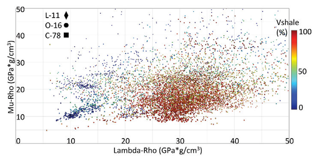
Figures 8-10 show crossplots in Goodway space coloured by Vshale for L-11, O-16, and C-78 for the Upper Jurassic interval for brine, oil and gas fluid saturation respectively. In each plot, two significant porous sand populations (low Vshale values in blue) separate from the shaley trend (red).

Firstly considering lambda-rho, as one might expect the effect of fluid fill is evident; lambda-rho values decrease as saturation is varied from brine to oil to gas for both of the porous sand populations. Additionally, lambda-rho is also a useful parameter in lithology discrimination. For each fluid scenario, the sand populations have low lambda-rho values (amongst the lowest values shown) and separate from the shale trends. Lambda-rho is less effective at separating porous sand from cemented sands and this is best seen in Figure 8. The cemented sands of L-11 and O-16 do not form a tight cluster, but are the scattered blue points at low lambda-rho and high mu-rho values, higher mu-rho than the upper porous sand trend. These observations are supported by the work of Hoffe et al. (2008), where interpretation templates show that high net-to-gross sandstones with low porosity due to cementation plot at low lambda-rho values and high mu-rho values.

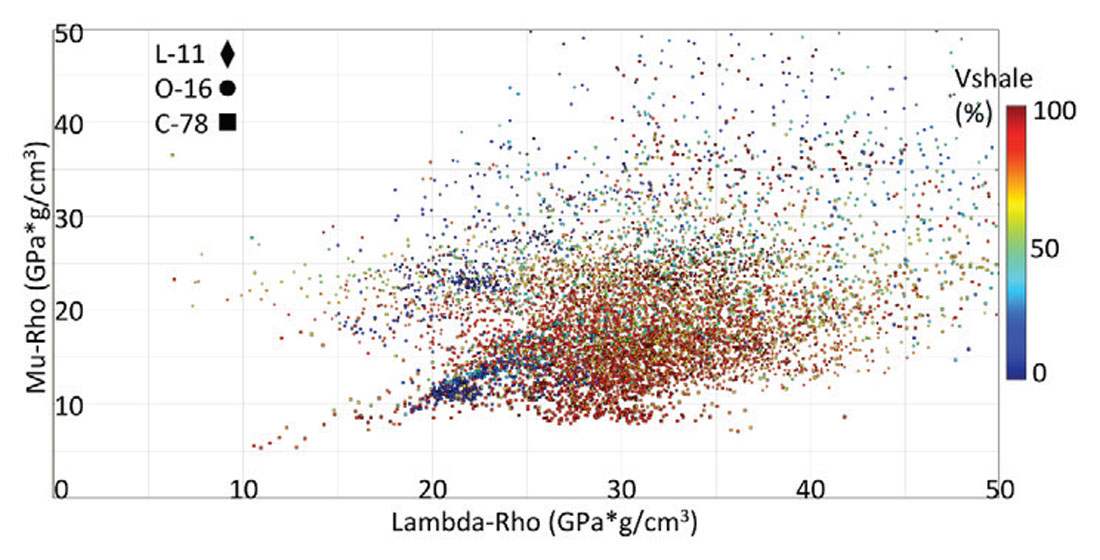
Mu-rho is typically thought of as a lithology indicator, and for these wells the porous sand populations separate into two distinct mu-rho trends. The low mu-rho porous sand population is primarily from C-78 sands and the upper sand in O-16, while the higher mu-rho valued sands are from L-11 and the middle sand of O-16. Both Vs and density drive this variation in mu-rho. Referring to Figures 2-4, and considering in particular the middle sands, it is observed that Vs values in C-78 are considerably lower than Vs values in L-11 and O-16. Vs values for the middle sand in C-78 are comparable to Vs values in over- and underlying siltstones and shales. In O-16 and especially L-11, the Vs values in the middle sand are considerably higher than the over- and underlying silty and shaley zones. In this example, porous sands and shales cannot be separated by mu-rho alone, as low and moderate mu-rho values correspond with both porous sand and shale populations. As mentioned, cemented sands can be isolated from porous sands via mu-rho. Similarly, carbonate lithologies (such as the limestones near the base of O-16, Figure 3) separate from sandstone and shale in lambda-rho mu-rho space. Carbonates are not abundant in these wells, but plot as the blue points scattered at high lambda-rho and high mu-rho values in Figures 8-10. These observations for carbonates are consistent with the lambda-rho vs. mu-rho crossplot templates in Hoffe et al. (2008).

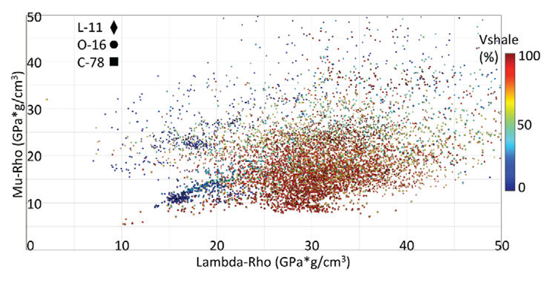
In general, lambda-rho vs. mu-rho crossplots can be used to effectively discriminate sandstone from shale and carbonates, hydrocarbon fill from brine fill, and cemented sands from porous sands. Lambda-rho seems particularly useful as in these examples it highlights both fluid fill and lithology. Thus these attributes offer less ambiguous information than reflectivity methods. However, it is worth noting that the porous sand/ source rock Class IV ambiguity is not fully clarified by these attributes. Again referencing Hoffe et al. (2008), a clean high-porosity sandstone will have both low lambda-rho and low mu-rho values, and could plot as a Class IV. In Goodway space this Class IV region is coincident with the position where low impedance shales such as source rocks may plot.

As shown in Russell (2014) and many other sources, it is also common practice to consider P-impedance (or acoustic impedance, AI) vs. Vp/Vs cross plots for fluid and lithology discrimination. It is anticipated that the P-impedance response will be directionally the same as both AVO intercept and lambda-rho and will aid in distinguishing lithology and fluids.

Vp/Vs offers an alternative lithology indicator to mu-rho and will also be influenced by fluid saturation.

Figures 11-13 show cross plots of P-impedance vs. Vp/Vs for brine, oil, and gas saturation respectively, all coloured by Vshale. A strong fluid effect is evident in these cross plots. Both P-impedance and Vp/Vs decrease from brine to oil to gas saturation; targeting low values in Vp/ Vs and P-impedance would be advisable for targeting hydrocarbon fill.

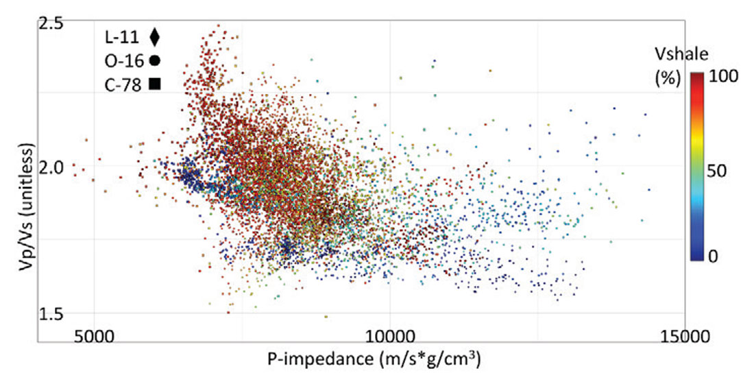
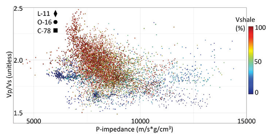
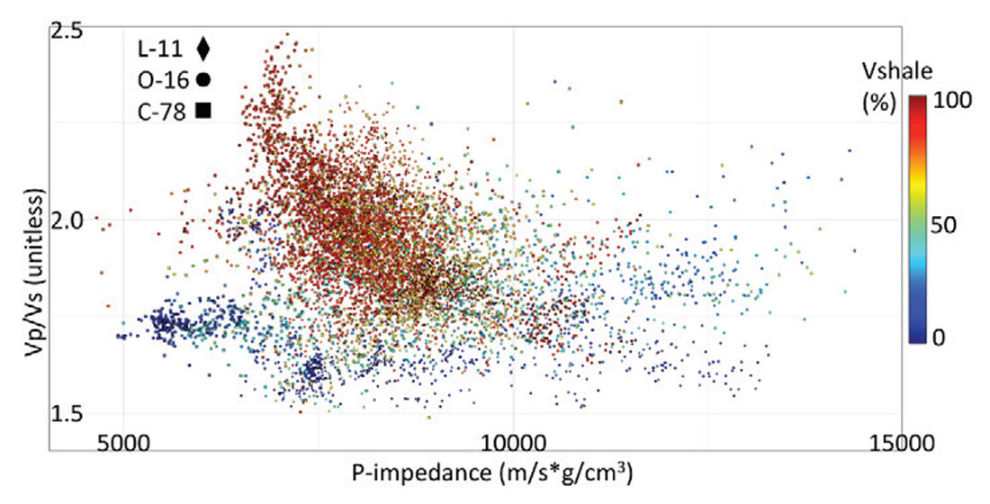
Lithology interpretation is also possible in P-impedance vs. Vp/Vs space. In Figure 11, the crossplot for brine saturation, two sand populations are evident. The sands at C-78 and the upper sands at O-16 plot at the lowest P-impedance values and at moderate Vp/Vs levels. Conversely, the L-11 sands and the middle sands at O-16 plot at the lowest Vp/ Vs values and moderate AI values. Additionally, the cemented sands in L-11 and O-16 and the carbonates in O-16 are scattered but generally plot at high impedance and low Vp/Vs values. Porous sandstones could be separated from shales and carbonates by isolating the low-to moderate values on each axis and dismissing the higher values as non-reservoir zones.

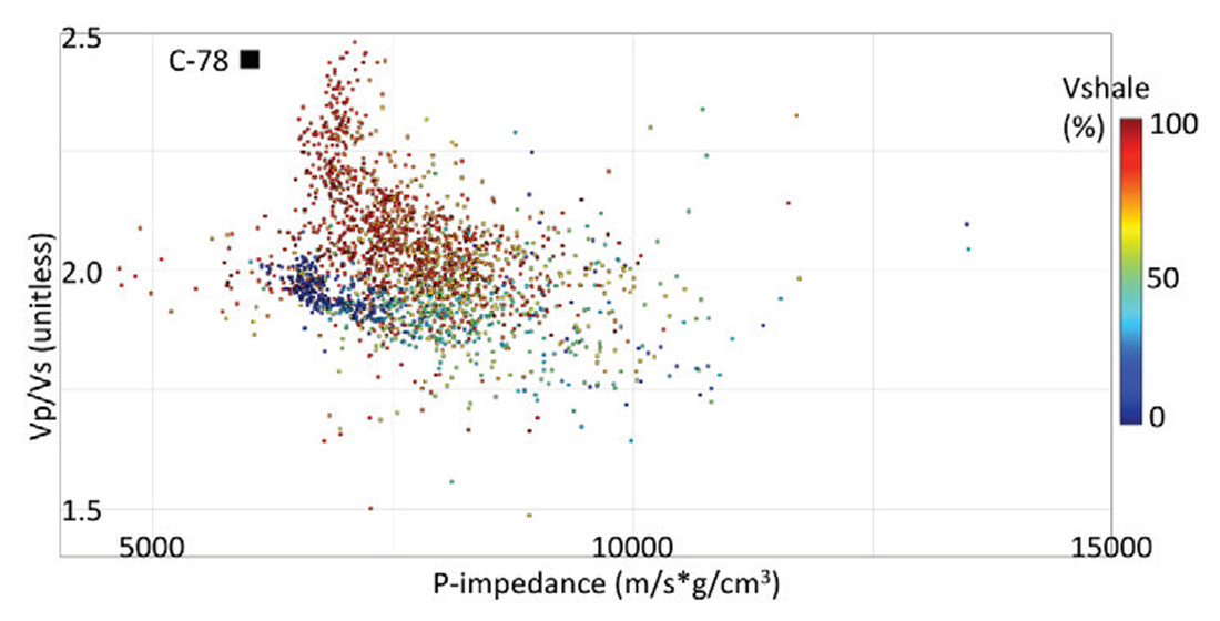
Figure 14 further clarifies the lithology discrimination. In this AI vs. Vp/Vs plot, only C-78 with brine saturation is shown. In this case the sandstones plot amongst both the lowest P-impedance and Vp/Vs values, compared with the over- and underlying Jurassic strata. Thus, on a local basis it might be acceptable to identify reservoir quality sandstones as having low Vp/Vs values, and low to moderate impedance values.

Discussion and Application to 3D Seismic Volumes

This log-based analysis provides useful direction for predicting lithology and fluids from 3D seismic volumes. A number of other Statoil workers including Rainer Tonn and Jo Bergen have contributed to this effort in the Flemish Pass, but their work has not been published.

The reflectivity methods considered can help in the identification of porous sand bodies and cemented sands and provide information about fluid fill. Careful modelling from local wells or inferring depositional environment from seismic interpretations might be required to resolve certain ambiguities such as discriminating thick, clean, porous sandstone from source rock, and in identifying thinner, low net-to-gross sandstone bodies. It could be argued that the nature of reflectivity analysis is somewhat ambiguous; defining the intercept value that justifies a change from a Class II to III, or gradient ranges that warrant a switch from Class IV to Class V are not obvious. Fortunately, the inversion methods analyzed resolve some of the ambiguities present in reflectivity-based analysis. Vp/Vs, and especially lambda-rho are capable of discriminating porous sands from shales and hydrocarbon saturation from brine saturation for the scenarios considered here. Thus these inversion-based attributes are considered very useful and are desirable products to guide prospect maturation and drilling decisions.

Given these observations, it is important to devise a strategy for reservoir characterization that may be applied to real 3D seismic data in areas tens of kilometres from well control. The ability of impedance methods to produce attributes similar to petrophysical logs is a clear advantage over reflectivity methods, thus inversions are preferred to reflectivity analysis. However, given that inversion methods typically require a background model that is calibrated to well data, one must exercise great caution if interpretations are carried significant distances, particularly into different sub-basins or into different play types. In such cases model parameters may be invalidated due to differences in lithology, mineralogy, pressures, fluids, burial depth, geological age, etc. In these cases, reflectivity methods based on general Vp/Vs relations or seismic processing velocities may be preferable, although ambiguities will remain.

An alternative that helps bridge the gap between the generality of reflectivity methods and the quantification of inversion methods is elastic impedance (Connolly, 1999) or extended elastic impedance (EEI) (Whitcombe et al., 2002). These methods operate on intercept and gradient data (reflectivity domain), thus they can be calculated from log data or prestack seismic volumes. Through coordinate rotations via varied angles, intercept and gradient volumes may be translated into new volumes in the impedance domain. The resulting products are considered representative of the relative changes in the given parameter; the products will have the same shapes, but not the same values, as the given impedance parameter. By applying different rotation angles, relative versions of attributes such as lambda-rho, mu-rho, and Vp/Vs can be produced. If well data are available, these relative values may be scaled to absolute. But in the exploration environment, it is useful to maintain relative values. In one EEI implementation for 3D seismic volumes used by Statoil, limited angle/offset stacks or intercept and gradient volumes are input. These input volumes can be created with seismic velocities, so well control is optional, but not required.

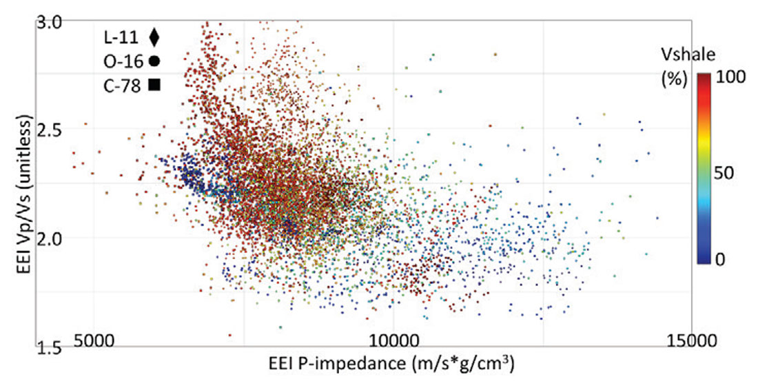
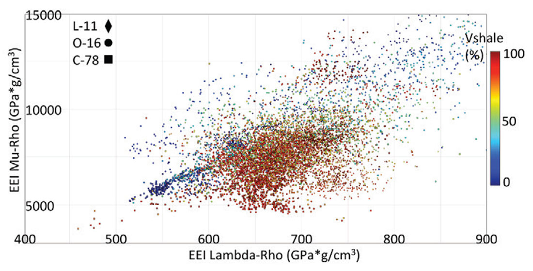
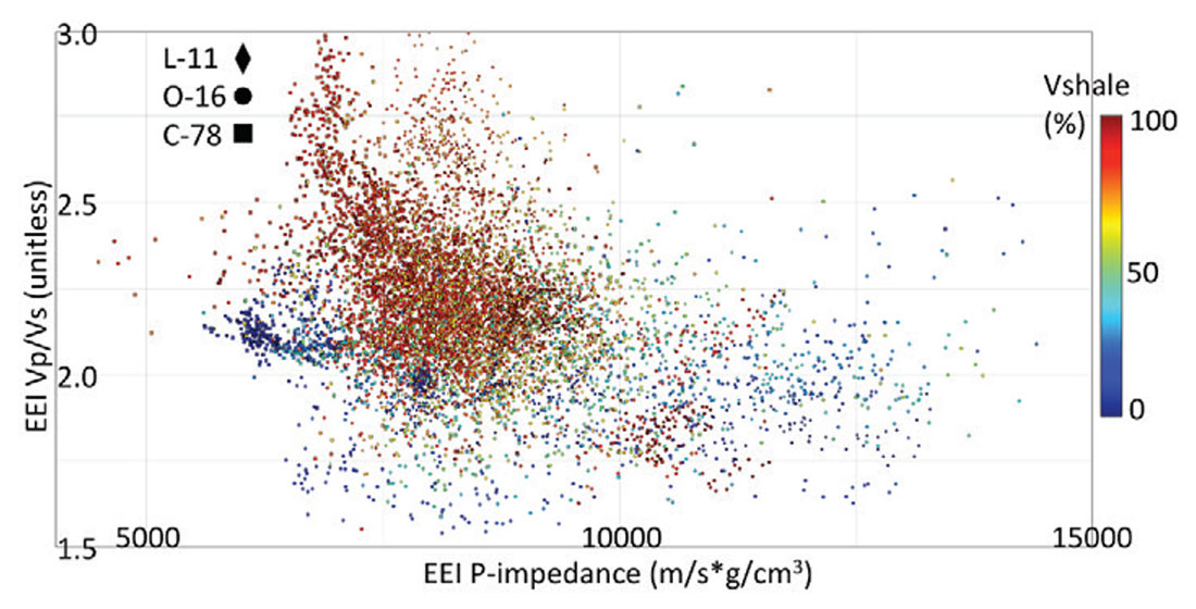
Figures 15 and 16 respectively show crossplots for the three wells of interest for EEI-derived versions of lambda-rho vs. mu-rho and P-impedance vs. Vp/Vs for brine saturation. The plots are coloured by the Vshale calculated from the log curves as for previous crossplots, although Vshale could also be calculated through EEI methods. These plots should be compared with Figures 8 and 11, the equivalent crossplots derived from log measurements, but the absolute values differ. For lambda-rho vs. mu-rho, the EEI crossplot shows a separation of the low mu-rho sand trend from the background shales via low lambda-rho values. The higher mu-rho trend does not separate from the shale trend. For P-impedance vs. Vp/Vs from EEI, the C-78 sands and upper sands of O-16 separate from the shale trends via low AI values. The other sands do not separate with EEI impedance, but separate via low EEI Vp/Vs.

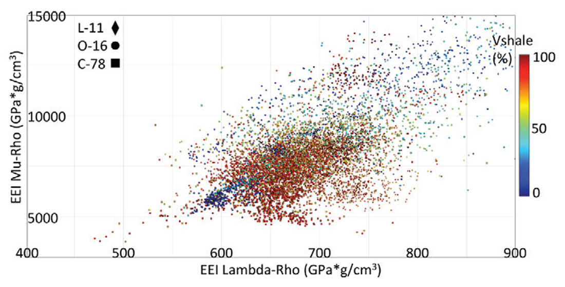
Overall, the sand from shale separation is clearer on the crossplots derived from log measurements rather than those calculated from EEI. However, there are great similarities in the measured log and EEI-derived crossplots, and similar interpretations might result from either method.

Figures 17 and 18 respectively show crossplots for the three wells of interest for EEI-derived versions of lambda-rho vs. mu-rho and P-impedance vs. Vp/Vs for oil saturation. These plots should be compared with Figures 9 and 12, the equivalent crossplots derived from log measurements, and 15 and 16, the EEI crossplots for brine saturation. For each EEI plot, the fluid effect of oil saturation is evident in reduced lambda-rho, P-impedance and Vp/Vs values compared with the brine cases. Thus fluid effects observed in measured fluid substituted crossplots are also observed in equivalent crossplots derived from EEI methods. Similar observations are made for the gas-saturated EEI data, but figures are not included.

The general diagnostic observations from the impedance-based log analysis were that low lambda-rho correlates with high porosity sandstones and hydrocarbon fluid fill, low to moderate Vp/Vs correlates with high porosity sandstones and hydrocarbon fluid fill and cemented sandstones have high mu-rho values. In the absence of absolute scaling, these relative values remain quite useful. This suggests that relative seismic attributes, those derived from EEI in particular, are useful exploration tools. While uncertainties and ambiguities remain, this method is very useful as it uses reflectivity data to produce impedance products without requiring inversion.

The recommended workflow in the exploration setting is to determine relationships from available well logs where possible. Appropriate impedance products can then be generated from seismic volumes via EEI methods. The interpretation of the variations in relative values can be guided by log data, analogue areas, or published guidelines.

Acknowledgements

We acknowledge Statoil for allowing publication. We offer special thanks to Statoil colleagues Elisabeth Mortlock for petrophysics and Rainer Tonn and Jo Bergen for their contributions to AVO methods in the Flemish Pass. We are also grateful for useful discussions with additional colleagues at Statoil and joint venture partners that helped shape this study.