A New Perspective on Shallow Water Flow (SWF) Prediction and the Prevention of Sinking Well-Heads in Deepwater Settings

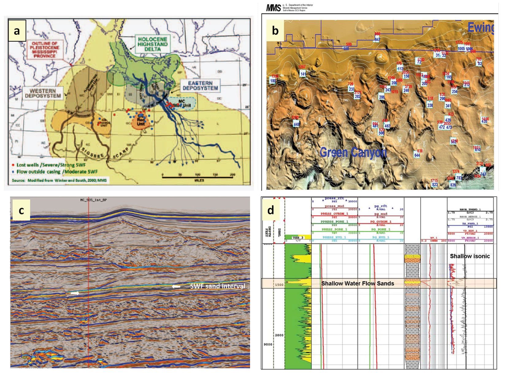
A new study integrating the seismic velocity profile with a proposed subsurface geopressure partition sheds light on a possible cause of shallow water flow (SWF) sands and sinking well heads in deepwater settings. The Bureau of Ocean Energy Management (BOEM), previously known as MMS, reported 157 cases of SWF in the Gulf of Mexico. Most of these cases occurred in the Mississippi and Green Canyons areas where a late Pleistocene depositional fan was active. Occasionally, surface casings and well heads sink and get lost in these areas as well.

Study of pressure gradient of sand vs. shale in the proposed subsurface zones (A, B, C and D) points to a possible source for these two events. The fragile nature of the unconsolidated shallow hydrostatic zone A is mostly responsible for the loss of the well heads. This shallow zone gradually transforms to a compacted hydrodynamic system (zone B), associated with a dewatering process that can lead to SWF.

Calculating the linear pressure gradient in the sand beds vs. the feasible formation pressure in the shale layers in zone B is the backbone of this shallow water flow study. The sand rapidly flows upward at a linear gradient ranging from 0.53 to 0.59 psi/ft. On the other hand, slow compaction of shale and dewatering follows an exponential pressure gradient. During drilling, penetration of the interface between the shale and the underlying sand causes sand flow that overcomes the mud pressure, and SWF takes place due to the pressure differential between the sand and the shale.

Mitigating these events should be attempted before drilling any wells in the deepwater. Seismic velocity, sequence stratigraphy and geopressure modeling can identify potentially problematic zones so that precautions can be taken to combat and avoid these challenges during drilling operations. Choosing the right depth for surface casing and adjusting the value of the mud-up during drilling to avoid SWF are recommended to avoid potential well abandonments.

Introduction

The causes of SWF were discussed in several previous studies. Mudline topography, shallow structural features, mud flows, gas hydrate expulsion and even very shallow over-geopressure are responsible for this phenomenon. Dutta et al. (2010) stated that “shallow water flow hazards can be characterized through deterministic indicators such as V_p /V_s ratios and density and also pore pressure that can be estimated quantitatively for the near seafloor sediments where conventional velocity analysis is not effective.” This paper introduces a quantitative fresh look at the shallow subsurface pressure profile zones that are related to geologic processes, and a new perspective of the prediction methods and algorithms.

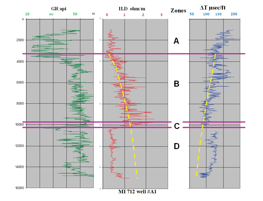
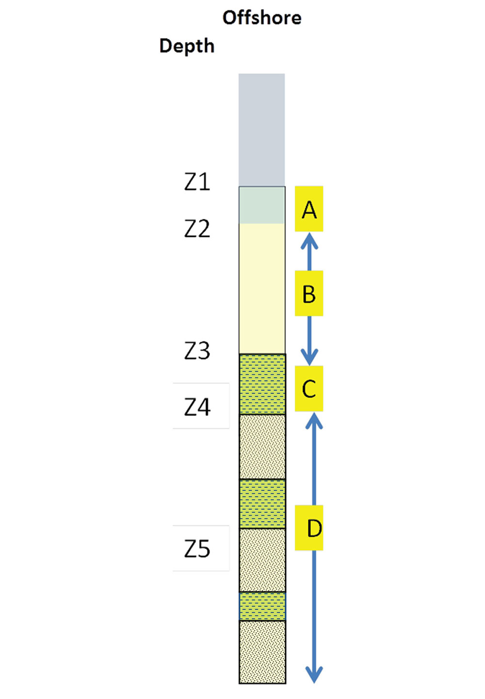
The vertical generic pore pressure profile in the subsurface can be, in most cases, divided into four zones (Shaker, 2012; Shaker, 2015) namely: free flow, hydrodynamic, transition and geopressured (A, B, C and D respectively). This is contrary to the inherited conventional assumption established by Fertl (1976) of two subsurface zones; namely hydrostatic and abnormally pressured. For the purpose of this article, only the upper two zones A and B will be discussed (Figure 1).

The free flow zone A is an extension of the hydrostatic gradient of the sea bed. Within zone B fluid starts escaping from deeper sediments to the shallower ones (hydrodynamic) and grain to grain contact increases. Fluid passage is contingent on subsurface geometry and lithology distribution as well as hydraulic conductivity (Bredehoeft and Hanshaw, 1968). The gradual reduction of porosity due to compaction is usually represented by an exponential trend (Figure 1). It is usually referred to, in pore pressure practice, as the normal compaction trend (NCT). It is suggested here that it should be designated as the compaction trend (CT) instead of the normal compaction trend, since the normal hydrostatic pressure is only observed in the free flow zone A.

Establishing the extent of the hydrodynamic zone B from seismic velocities is crucial to pressure prediction. The depth to the start and end points of zone B is contingent on the lithofacies, overburden, and any tectonic or structural stresses. The depth to the stress that can choke the low permeability sediment and prevent any further fluid expulsion is referred to as the top of geopressure (TOG). Fluids cease flowing at the base of zone B (top of geopressure transition / zone C).

Hydrogeology – formation pressure

The Mississippi delta was very active during the Pleistocene time with high rate of sedimentation into the Mississippi and Green canyons areas (Figure 2). Thick clastic sediments, mostly shale, clay and sand, sometimes reaching 10,000 ft thick, were deposited over the last 1.7 million years. The compaction process of these deposits is still active, and the continuing dewatering is significant.

Zone A

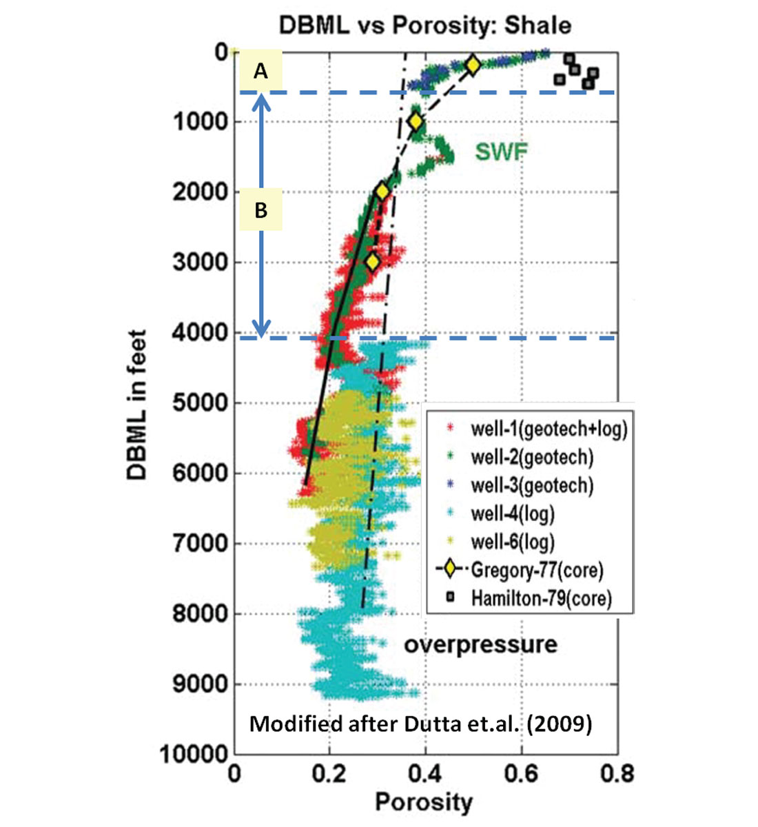
In this zone, the depositional environment receives sediments as debris flow with over 50% water saturation. Galloway and Hobday (2000) stated that during the first 1000 ft of burial, mud releases over 21,000 cm³ of interstitial water per cm² of surface area, and porosity is reduced from over 50% to about 35% (Figure 3). Rubey and Hubbert (1959) stated that for depths of 1 to 2 km, pressure is a function of depth where fluid moves freely and exhibits a hydrostatic pressure gradient derived from the weight of the water column only. Zone A’s pressure gradient in the Gulf of Mexico is 0.465 psi/ft (10.52 MPa/km).

The loose coupling of grains and the high pore volume filled with formation fluid impacts both velocity and resistivity. In zone A, velocities stay in the range of 5000 – 5500 ft/sec. Fluid resistivity in this zone is dependent on salinity, and ranges from fresh water to brines, contingent on the proximity of a fresh water source (Figure 1). In south Louisiana, the average resistivity measurement is about 1 ohm (Ham, 1987) from the surface to depth of ~4000 ft. This indicates a large extent of zone A with an abundance of brackish water.

Driving the 36 inch casing into the sea bed is a common practice due to the unconsolidated nature of zone A.

Zone B

This zone starts at a depth where the overburden’s stress promotes the fine sediments to start the process of dewatering (Figures 1 and 3). This phenomenon can be observed in most of the shallow subsurface sections due to the reduction of porosity with depth. Fine clastic sediments, especially shale, lose most of their formation water, except for interstitial and bound water, during this process.

The mathematical model of Smith (1970) with negligible permeability at the base (i.e. a seal) shows a gradual reduction in the water flow rate and, conversely, an increase of pore-water pressure that coincides with an increase of overburden and matrix frame pressure. This is consistent with the presence of hydrodynamic upward flow in zone B and the assumed minimal permeability in zone C. The upward hydrodynamic gradient is usually greater than the normal hydrostatic gradient (Dahlberg, 1994; Shaker, 2012).

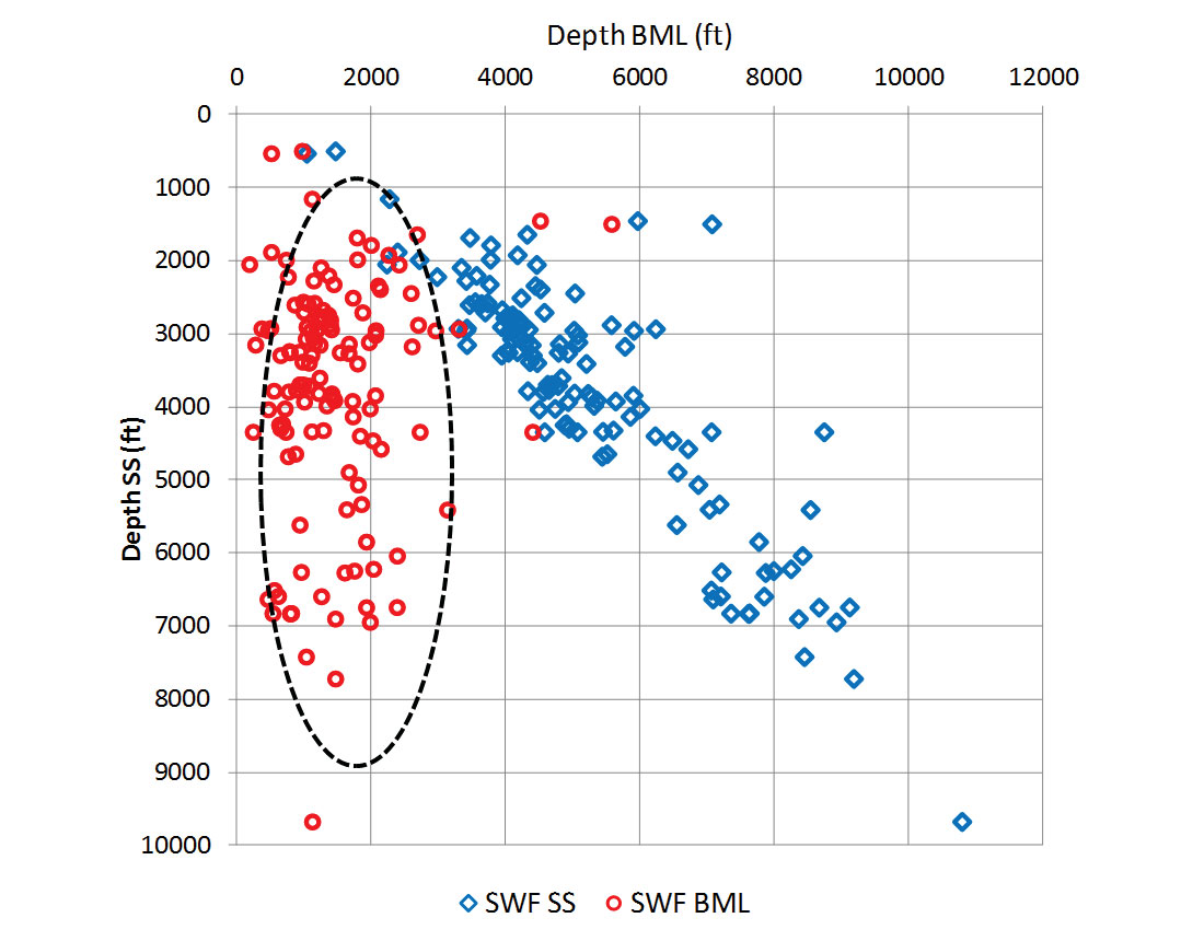
The fluid flux throughout the sediments, from deep to shallow, due to the dewatering process, sometimes gives the impression of a shallow/near surface geopressured zone. This is common in the deepwater environment at depth ranges from several hundred ft to 3500 ft below the mudline (Figure 4). It occasionally causes drilling hazards referred to as shallow water flow (SWF) if mud weight is not programmed to combat the sand’s flow surge. Dutta et al. (2009) stated in their study “Figure 4a shows an interval of anomalously higher porosity than the background at 1500 ft. This interval corresponds to the overpressure regime due to the presence of SWF.” Their Figure 4a is modified in this article as Figure 3. Huffman and Castagna (2001) noticed that the SWF occurs at depths of 4000 ft below the mudline due to different physical properties and is present “near the transition between rocks and sediments.”

Shallow water flow occurs in wells drilled at subsea water depths ranging from 1000 ft to 8000 ft. The water flow mostly takes place at average depth range from several hundred ft to 3500 ft below the mudline (Figures 2, 3 and 4). The relationship on Figure 4 indicates that the cause of SWF is independent of subsea water depth. Therefore, litho-stratigraphy associated with overburden stress that causes the flow rate changes are the driving mechanism behind this phenomenon.

The slope on petrophysical measurements in zone B represents the compaction trend (Figure 5) and should have a unique slope and extent for a specific location (e.g. common depth point, seismic gather). The aforementioned facts shed light on a very important case that validates the inaccuracy of using effective stress theorem to predict pressure in zone B, where the grain to grain coupling is not fully achieved. The concept of effective stress, to predict pore pressure, truly becomes divisive when dealing with non-hydrostatic (i.e., hydrodynamic) pore water pressure. Dutta et al. (2010) called for a method that can quantitatively estimate the pore pressure for the near sea floor sediments where conventional velocity analysis is not effective. Multi-component technology, in spite of its limitations, can yield V_p/V_s ratios directly. However, deriving V_p/V_s from inversion of 3D seismic data is more cost effective and valid in all submarine conditions.

Predictive modeling before drilling

Defining zones A and B before drilling:

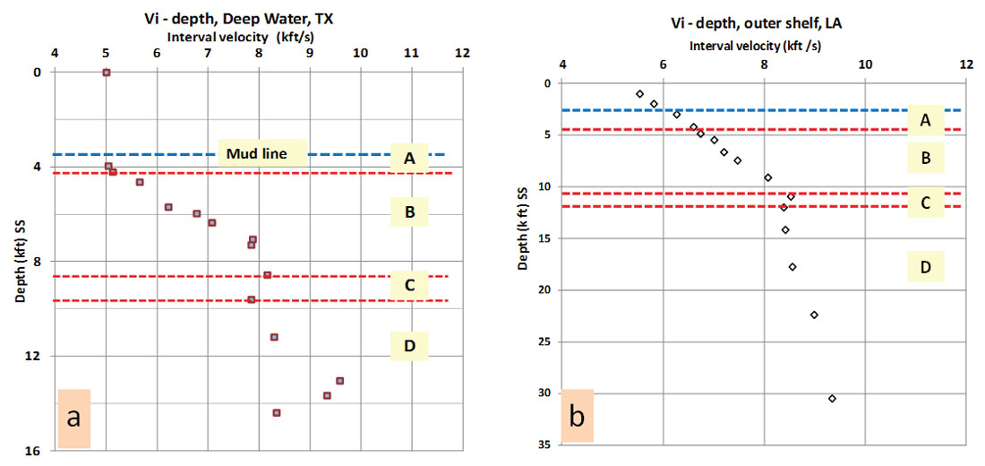
Compressional seismic velocity (V_p) is the first petrophysical property that can be used to predict the depth to zones A and B, and the top of zone C. Normal moveout and RMS velocities can be used for a quick look and regional assessment. However, interval or Dix velocity (Vi) is the velocity recommended for 1D and 2D interpretations. Quality control displays such as NMO-corrected gathers should be used to check the accuracy of velocity picks but never to make predictions based on single velocity function. Velocities must be processed for de-multiple, DMO (dip move-out) and pre-stack migration. Converting time-velocity pairs to depth-velocity pairs is required and needs to be calibrated against check-shot, velocity survey and/or sonic logs from offset wells. Outlier velocity values representing calcareous beds, salt inter-beds, gravel, thick sands and pay zones should be eliminated from the analysis. Figure 5 shows velocity pairs from two depositional environments, deepwater and flexure trend / outer shelf, and the estimated depth for each of these zones.

In zone A, the velocities average ~5000 ft/sec (~200 μs/ft). In zone B, the data values show a gradual exponential increasing trend on a linear scale (Figures 1 and 5). The pivot point where the velocity trend changes course from increasing to decreasing with depth is the approximate depth to the base of zone B.

Calculating pressure in zones A and B:

It is assumed that there is an offshore deepwater wildcat trajectory and pressure will be calculated at specific depths in each zone (Figure 6).

At the mudline:

where ρ = density of seawater; g = gravitational acceleration; z₁ = water depth; and 0.4335 is the pressure gradient conversion from 1 g/cc to 1 psi/ft .

Calculating pressure in zone A:

The top of zone A is at the mudline (z₁) and the base (z₂) is where the velocity values begin the gradual compaction trend. Zone A is where porosity ranges from 50% to 30% and velocity is responding to the fluid (Figure 5). Pressure (psi) at the base of zone A is given by:

where ρ = density of shallow formation’s water (≈ sea water).

Log measurements are frequently unavailable due to the driving of the surface casing string (36 inch) into zone A. The surface casing and well head sometimes sink and get lost in this fragile zone e.g., Mississippi Canyon block 711 well #2 and block 755 well #1, Green Canyon block 854 well #1, and Atwater block 362 well #1.

Pressure calculation in zone B:

All the previous methods calculate the pressure in zone B as if a normal hydrostatic pressure exists. In this paper a new estimation method is introduced to calculate pressure in this hydrodynamic zone. The hydrodynamic pressure value at a certain depth is a function of permeability and differential pressure between the bottom and top of each compartment in this zone. The pressure estimation in B zone follows Darcy’s Law. However, Darcy’s law is probably more applicable in the laboratory than in a complex geologic setting. This is due the presence of multiple lithologies with different permeabilities, and the complexity of assigning the values of entry pressure for the system. The discharge segment B begins when and where the fluid pressure exceeds the hydrostatic gradient due to the increase of sediment load, grain to grain contact, and in situ pressure. The effective stress theorem is applicable only if fluid is at rest (hydrostatic gradient) and is not flowing (e.g. stage A in Terzaghi and Peck’s 1948 model where λ = 1). Empirical correlation between velocity trends in the so-called normal pressure section (zones A and B) and ΔP was not important according to these earlier studies. This is a result of the assumption that the entire section above the top of geopressure (TOG) is hydrostatic and normally pressured.

Calculating the pressure in this zone is an intricate mission, especially in a wildcat area, since it requires offset data for calibration. The top of zone B starts when the velocity exponentially increases in response to the decrease of porosity with depth following Athy’s relationship (Athy, 1930). The top of zone C (bottom of B) starts when the velocity trend reverses its course (Figure 5).

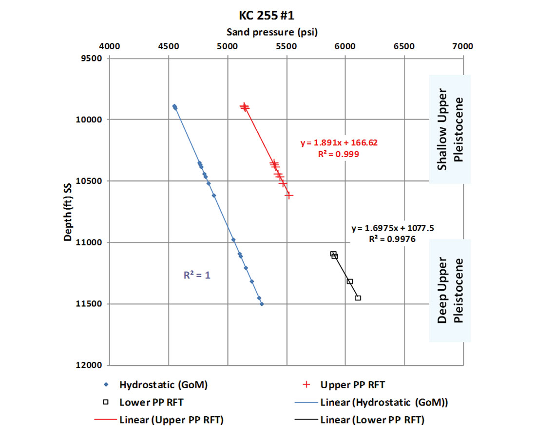
Occasionally, repeat formation tester (RFT) and modular formation dynamic tester (MDT) measurements are taken from this zone’s sand beds in deepwater wells in the Gulf of Mexico. They show a clear upward hydrodynamic flow (Figures 7 and 8) with a higher gradient than the GOM hydrostatic gradient, and exhibited hydraulic head reaches above the mudline (Shaker, 2012).

Mud weight (Figures 9a, b, c and d) increases from 8.9 ppg at the top of zone B to a value sometimes exceeding 11.5 ppg at the base to counter the up flow. An intermediate 9 5/8 inch casing seat usually set in the shale section of the pressure ramp at the base of B zone (TOG).

Pressure in sands:

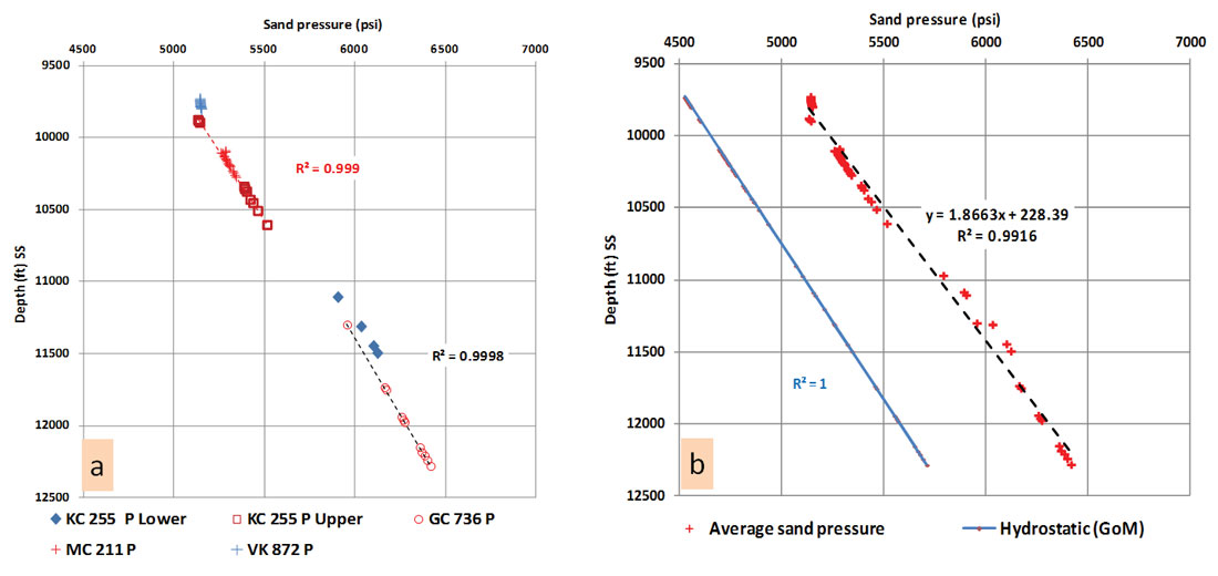
The purpose of establishing the empirical pressure-depth relation in this study is to predict pressure as a function of depth in the hydrodynamic zone. In the deepwater of the Gulf of Mexico, the sand pressure gradient in this zone ranges from 0.53 psi/ft (10.2 ppg mwe) to 0.59 psi/ft (11.4 ppm mwe) with an average gradient (Figure 8b) of 0.54 psi/ft (10.4 ppg mwe). This calculation was made using deepwater wells with pressure measurements in sand beds in reference to subsea. The least squares fit for all the sand data measurement are linear with R² values of 0.99 (Figures 7 and 8). This is in agreement with the flow nature of a sand bed that has a pressure gradient greater than hydrostatic (0.465 psi/ft) and can flow above the mudline if sand flows freely – i.e. when not capped by drilling mud pressure.

The sand pressure-depth relation of Keathley Canyon 255 plot (Figure 7) shows a gradient of 0.53 psi/ft (slope) and a hydraulic head (intercept) of 167 ft below sea level (~5630 ft above mudline) in the shallow Upper Pleistocene section. On the other hand, it exhibits a gradient of 0.59 psi/ft and a hydraulic head of 1077 ft below sea level (~4723 ft above mudline) in the lower section. This confirms the up flow of the sand beds in the B zone. Moreover, the upper section is more buoyant than the lower section.

An average trend in this study is calculated based on several available sand pressure data sets from four areas in the deepwater of Gulf of Mexico (Figure 8b). Measured pressure data collected from Mississippi Canyon (MC), Green Canyon (GC), Keathley Canyon (KC) and Visco Knoll (VK) are used. The gradient in the Pleistocene deeper section in KC and GC areas shows higher values than the shallow Pleistocene section in the KC, GC and VK areas. This also confirms the general regional upward flow where the lower gradient fluid has more buoyancy than the higher gradient fluid and where SWF is common in the shallow Pleistocene section. The overall data values for the above mentioned areas (Figure 8b) show an average gradient of 0.536 psi/ft and hydraulic head of 230 ft if sand flows freely to the sea floor (mud pressure is absent). Figure 8b also shows that the average pressure gradient of the sand beds is greater than the normal GOM hydrostatic gradient. Predicting the sand’s pressure in this zone is important to avoid any unexpected flow during drilling.

Solution for equations on Figures 7 and 8 gives:

Sand pressure in the shallow Upper Pleistocene at depth z₃ can be calculated as:

Sand pressure in the deep Upper Pleistocene at depth z₃ can be calculated as:

Average Upper Pleistocene (psi) at any depth (z₃) within the B zone can be calculated as:

Mud pressure gradually increases to compensate for the pressure differential between the high flow sand and the low permeability negligibly-flowing shale. Pressure in sand follows a linear upward flow (equations 3, 4 and 5) and the shale pressure follows an exponential trend (Figure 9d) reflecting the reduction of porosity (Athy, 1930). Usually, mud weight is raised at the shale-sand interface where drilling events requires mudding up.

Pressure in shale:

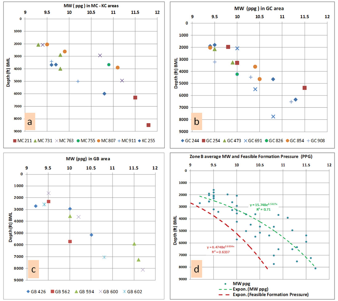
Calculating the average formation pressure of shale (feasible formation pressure) in this zone is estimated from the populated MW data sets. The mud pressure (ppg) at any depth (z₃) within zone B is calculated from mud weight values of Mississippi Canyon (MC), Keathley Canyon (KC), Green Canyon (GC) and Garden Banks (GB) areas (Figures 9a, b, and c). On these plots, the depth value data (y axis) are in reference to the mudline due to the wide range of subsea depths to mudline. The average mud pressure (equation on Figure 9d) required for keeping the borehole stable and avoiding any formation water flow follows an exponential trend. The least squares best fit for the data ranges from 9.15 ppg to 11.7 ppg, and can be calculated as:

The constant α for this data set is 5.18 (R² = 0.71).

Equation 6 was calibrated and validated using known mud weights from numerous offset wells.

The estimated average feasible formation pressure (FFP) was gauged by mud weight pressure data from wells drilled with balanced mud and where SWF were not reported. It is also based on the drilling practices and safety regulations that are constrained by formation and fracture pressures. Mud weight is usually 0.5 ppg greater than the before drilling predicted pore pressure at the second casing string (20 inches) and is 0.75-1.0 ppg greater than predicted pressure at 16 – 13 3/8 inch casing strings and the intermediate casing. The average FFP therefore follows the same exponential trend (Figure 9d) and can be calculated at any depth below the mudline (z₃ – depth ML) in zone B as follows:

Feasible formation pressure in ppg mwe = 1.49 ln (z₃ – depth ML) – α (7) where constant α is 2.79 (R²= 0.63).

Prevention of shallow water flow (SWF)

The objective is to calculate the pressure difference between the sand flow (equations 3, 4 and 5) and the average feasible formation pressures (equation 7) to avoid unexpected SWF sands. Calculating the pressure difference between the sand flow and the FFPin psi at the shale – sand interface foresees the required MW increase (mud-up) to combat the SWF without loss of circulation and avoid the flow-kill-breakdown (FKB) cycle. For example, the difference between the average sand pressure and shale FFP at a sub-sea depth of 10,000 ft and water depth of 5830 ft is:

Sand pressure at 10,000 ft (SS) = (10⁴ x 0.536) – 123 = 5237 psi (from equation 5) = (5237/10⁴) x19.3 = 10.11 ppg mwe

FFP (4170 ft BML) = (1.49 x 8.335) – 2.79 = 9.64 ppg (from equation 7)

Therefore, the mud-up required at the shale-sand sequence interface is 10.11 – 9.64 = 0.47 ppg (~0.5 ppg). Additional mud-up may be required in case of high connection gas associated with penetration of the sand-shale interface (contingent on the leak off test at the casing point above this depth).

The mud-up needed for the shallow Upper Pleistocene section at a depth of 10,000 ft (SS) is 0.41 ppg (equations 3and 7). On the other hand, mud-up is almost negligible at 12,000 ft (SS) as it is only 0.13 ppg (equations 4 and 7). This confirms the observation that the Upper Pleistocene shallow section is more hazardous than the deeper section, and that SWF usually occurs between several hundred ft and 3500 ft below the mudline.

Summary and recommendations

The newly introduced SWF prediction method before drilling is valid and applicable in the Pleistocene section of the Gulf of Mexico. It can also be successfully applied in other deepwater settings worldwide where relatively young sediments were fed into basins through major deltaic systems, such as the Nile and Niger Deltas, and also south Asian areas.

Application for pore pressure prediction:

1. Delineating zones A and B using seismic velocity is a keystone for any pre-drilling shallow hazard prediction.
2. Shallow water flow is independent of mudline’s water depth and is governed by lithostratigraphy and compaction due to the overburden load.
3. One of the main possible causes of SWF is the pressure difference between the high linear sand flow and the very slow exponential shale flow due dewatering in zone B.
4. The assumption that the sedimentary section above the top of geopressure (i.e. zones A and B) is hydrostatically (normally) pressured can lead to unexpected SWF.
5. Empirical depth-pressure relationship should be established to predict pressure in the hydrodynamic zone B, instead of considering it as a hydrostatically pressured zone or applying one of the effective stress methods.
6. The gradual reduction in porosity during the expulsion phase (zone B only) impacts petrophysical properties (V, R, ρ, etc.). The exponential trend line that connects the data points, in zone B, should be called the compaction trend instead of normal compaction trend.

Application for drilling practice:

1. Investigate the possible deeper extension of the surface casing (36 inches) to zone B in order to avoid well head sinking.
2. Estimating the mud-up value at the shale / sand interface is essential to prevent SWF and avoiding the FKB (flow-kill-breakdown) cycle. Studying this relationship and defining the hydraulic head above the mudline, especially in the shallow sequence of the Upper Pleistocene in MC and GC areas, can result in avoiding the abandonment of several locations due to SWF.
3. Estimating the depth to zones A and B from seismic velocity can be done in conjunction with sequence stratigraphy and high resolution seismic in the Pleistocene section to pin point the shale/clay – sand interface. Shallow geological features (e.g., shallow faults and mudline gouges) can exacerbate this phenomenon.

Finally, this is a new tool can be added to a list SWF prediction methods which includes V_p/V_s, 3D inversion modeling, and multi-component techniques.

Acknowledgements

The author is indebted to Dr. Rob Holt and Satinder Chopra for their reviews. Moreover, thanks also go to Dr. Barry Katz and anonymous reviewer #3 of the Interpretation Journal for their appraisal of the expanded article “A new approach to PPP”. The author also acknowledges the BOEM (previously MMS) staff for their generous online database.