White Noise Suppression in the Time Domain

Summary

White noise forms the basic limit to resolution for seismic data. However we are not usually trying to see a single event on a single trace. We recognise that seismic signal “looks” the same within a time window at least on some adjacent traces. We can use this to nonlinearly progressively remove the signal and what is left is then the noise which we can remove from the original section.

Two modules (4d,5dDEC) for removing white noise from seismic data will be presented. They employ principal component decomposition in the time domain. (Jones – 1985) Because all frequencies move together in a spatial sense, this domain offers a considerable advantage in processing the low amplitudes at the top end of the wavelet’s spectrum. It will be shown, with the aid of cross correlations, how one can recover most of the signal respecting curvature in space and statics down to about 30dB with only a few basis functions (which are the elements of the principal component decomposition). The original amplitudes are preserved and the noise is removed without mixing. Finally, examples will be shown to illustrate that this process really does work and how it can be used to enhance seismic processing.

In short if you respect that seismic data “wobbles” in space and changes amplitude, then the seismic signal may be extracted relatively easily.

Introduction

This topic has received a lot of attention recently in the guise of trace interpolation. (Lui et al– 2004). To interpolate a trace you must first extract the signal on adjacent traces and that is what we are doing with this method. However that work was done principally in the frequency domain. That has proven difficult and I believe unnecessarily so. Considering the amount of work that has been done in this domain I trust that I do not offend.

Part I

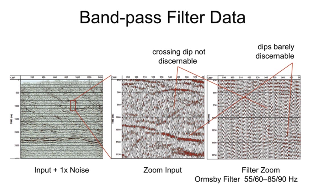
The frequency domain has three major disadvantages. First the signal energy falls off at higher frequencies so dip determination there becomes problematic. Of course the lower frequencies can be used to guide the higher but that introduces further problems. The second problem is that these higher frequencies tend to alias. [see: crossing dip] The third and more systemic problem is that the basis functions are linear. Seismic data, even when restricted to small windows, is curved and more important it “wobbles” in both amplitude and statics. This scatters energy into basis functions that have little to do with the primary signal. We assume that the signal is smooth and continuous (premigration) but I wonder is this ever really true?

So it was decided to rework the problem in the time domain. This domain is handy because all the frequencies move together in space unless we have dispersion. The latter we can deal with by operating in relatively small (say 21 traces by 300msec) windows overlapping in time and space.

Theory and/or Method

It is important to realize that white noise is random and hence unpredictable. Our job therefore is to attack and remove the signal which is recognized because within small windows some of the traces “look” the same. They move up or down dip, change amplitude and jitter up and down (because of statics) but still “look” the same. Conflicting dips may be removed with successive passes.

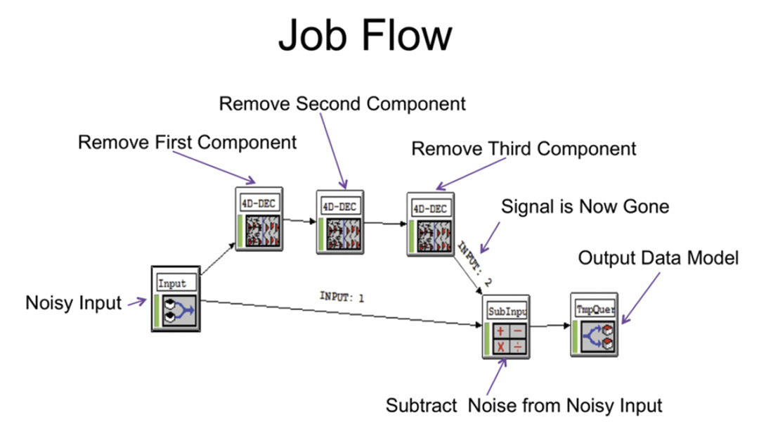
We take the data remove up to 3 different dips at any single time and place and subtract this from the input to get our final noise removed section.

Here is a real example (see Figure 3). The window is 21 traces by 300msec. In the second/third window you can see how the strong dipping event rattles up and down and changes amplitude. Why it does this we can speculate on but it definitely is doing it. The fourier transform of this would indeed be messy.

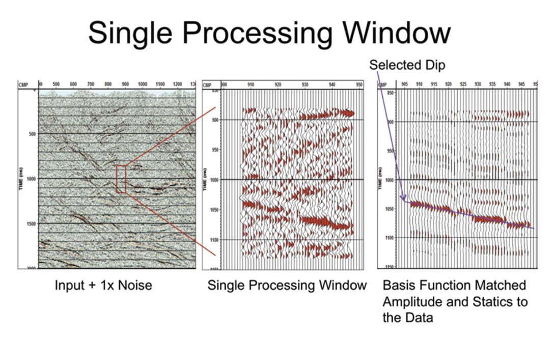
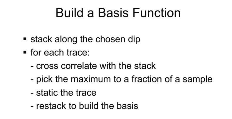
Figure 4 below shows how to build a basis function (which is a trace that “looks” like the data). The principal dip is identified by stacking along all possible dips . The stack traces are raised to the 4th power and summed to identify the dip that gives the sharpest stack.(minimum entropy) Because the data is only approximately linear this stack is low frequency. So we now cross correlate each trace with the stack, static it and restack to yield a high frequency basis function. Note that if some high frequencies are lost at this point, they will never be recovered. That is the residual signal will be too weak for subsequent passes to detect.

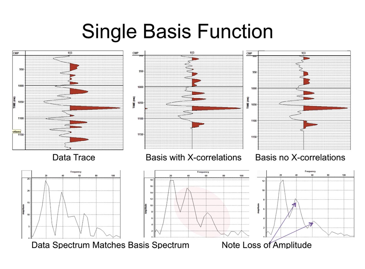
Typically the cross correlations are limited to about +-25msec but more has been used without seeing leg skipping effects. Though it is not entirely apparent on this plot, the basis with cross correlations has an amplitude spectrum that matches the data spectrum even out to 80Hz and 30dB down. More evidence of this is available in Part II.

Now this process is interesting. Potentially if you were to take a constant wavelet and add white noise, then when we build the basis the result could be a sharper wavelet than the original. (The noise may be richer than the wavelet in high frequencies.) For data in which the noise is the same amplitude as the signal we do not see this effect, but when the noise is say seven times the signal then the effect is visible (see Part II Figure 3). This implies that even though all frequencies move together, as the noise increases, there is a point where the high frequencies are being lost.

Also this process depends on reducing the noise through stack. If some of the noise is strong and not white it will overwhelm the stack and force the program to use the first pass to remove it. In practice, a different algorithm THOR based on median filtering is used to remove this strong noise before we run the algorithm described here. Note also that the stacking reduces noise by square root of the number of traces in the window. Too long a window will result in statics exceeding the allowed range.

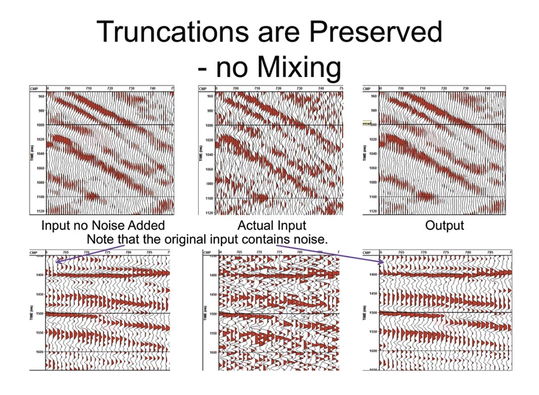
Now that a high frequency basis function has been found, it can be matched in amplitude and statics to each trace in turn – as was shown in Figure 1. It is then subtracted from the original data. Note that if the original event truncates abruptly (say after migration) then the amplitude match will zero the basis contribution just as abruptly. There is no smearing of the data and the output will match the input signal amplitude (see Figure 1). To reiterate: if only a third of the traces in the window have signal on input then only one third of the traces will have signal on output.

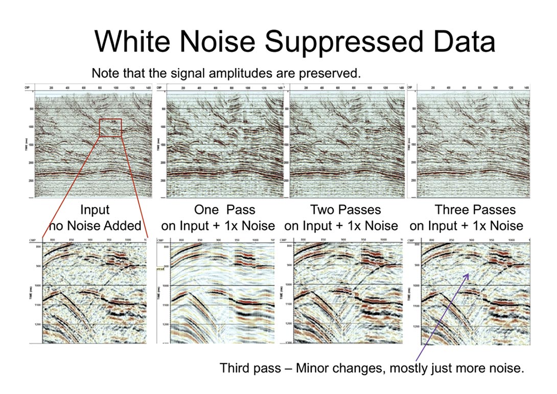
These windows are tapered and overlapped to cover the whole section. After one dip has been removed this process can be repeated until all the visible signal is gone. In practice three passes are usually sufficient. When the signal is gone this residual is subtracted from the original to get the enhanced section.

Examples

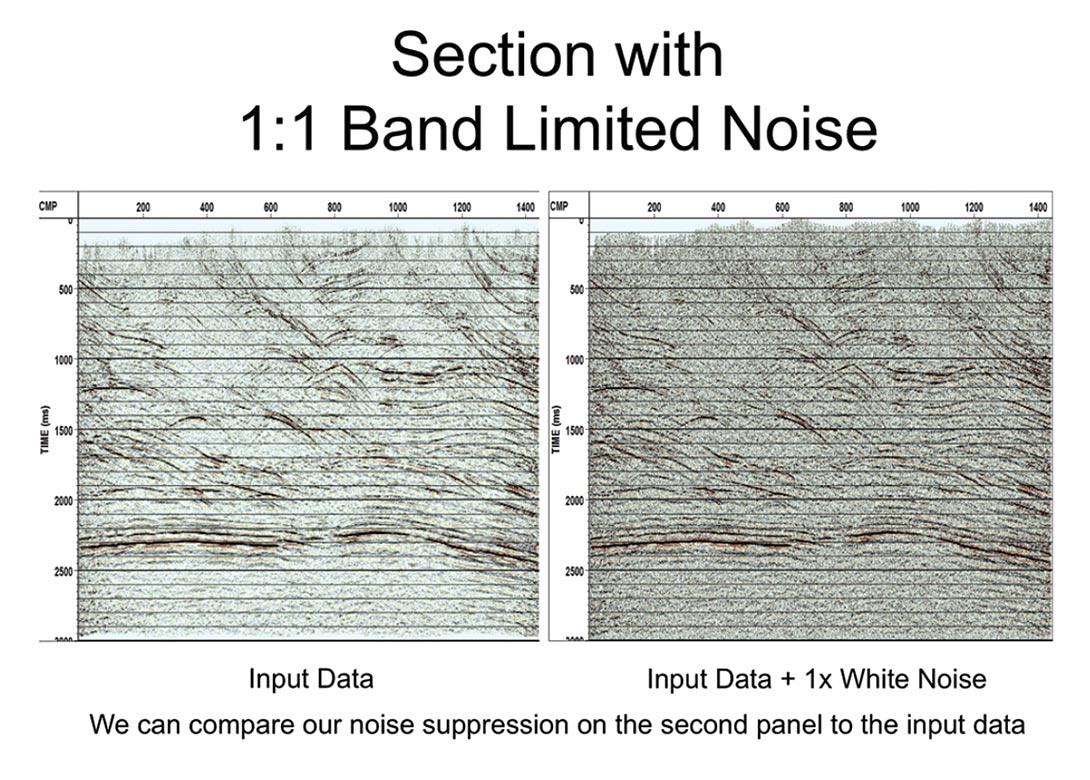
To test the algorithm a stack containing some noise is combined with white noise band limited to the signal frequency range. The RMS amplitude of the noise is equal to that of the original data – as shown in Figure 5.

In Figure 7 the results of processing the input data + 1x white noise are shown. The left most panel is the original input data. A window of 21 traces was used. (4.6x noise reduction). Note that in using 3 basis functions a simultaneous solution should be used, but in practice successive subtraction is good enough.

The first pass picks up only one dip. Note that though we have only one dip at any point we can shift from dip to dip very quickly and smoothly (the windows are overlapped and summed.) The second pass has two dips and creates character changes on the first dip. The third pass gets character changes on the secondary dips and any remaining third dips. In most parts of the section, however, it is just adding more noise. Note that we have some data being brought out that is barely visible on the original. The program is not only removing the noise we added but also noise on the original stack.

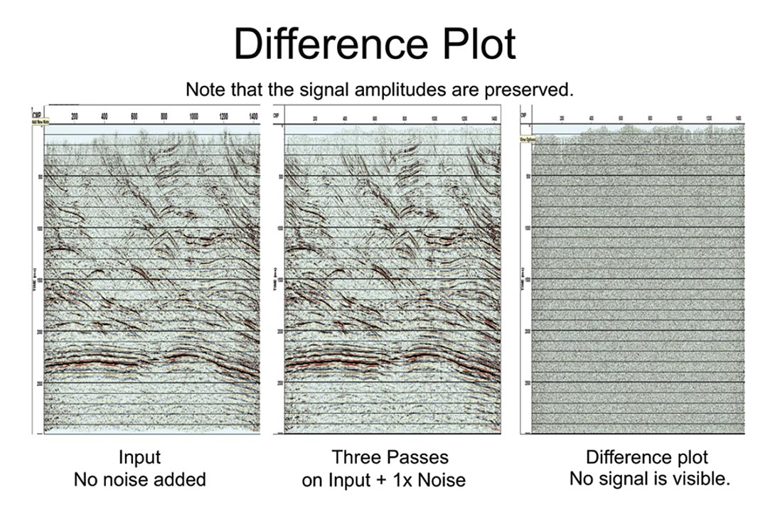
This next slide shows you a difference plot for reference but please note that the effects we are going to look at are far below anything you can easily see on the difference.

Now it might seem odd that we are able to match the signal so well and so easily with so few basis functions (see Figure 1 as well as the Figures below). Part of the answer lies with the amplitude/ statics matching, part of it is just that seismic signal does not vary that much laterally (frenel width – seismic spatial resolution), part of it is that the geology tends to be consistent over at least some of the traces, part of it is that we are using high resolution basis functions and part of it is that the wavelet can change because we are overlapping and superimposing windows.

In Figure 9 the events are examined in detail. The event truncations are not smeared by even one trace. Event amplitude and character are preserved. The output is not identical to the original input but this is mostly because the original input contains some noise.

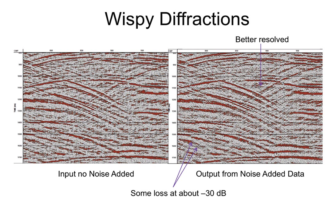
In Figure 10 we examine the effect of the algorithm on diffracted energy – particularly when that energy is very low. There is some loss on the wispy diffractions about 30dB down. However some has been gained too. This limit is dependent on the square root of the number of traces used to create a basis function. The data may or may not support longer windows.

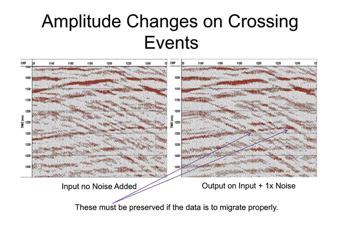
The amplitude changes as events cross are shown in Figure 7. These must be preserved if the data is to migrate properly.

Please note that these programs are not only very high fidelity but also extremely fast to run. Suprisingly this simple solution really does work.

Conclusions Part I

This concludes the first part of my paper. We have shown that the signal can be modeled with a small number (up to three) principal components in the time domain. The frequency content, amplitudes and fine structure of our original signal has been preserved in the presence of a moderate amount of noise [S/N ~ 1.0] down to a limit of about 30dB. In short if you respect that seismic data “wobbles” in space and time and changes in amplitude, then the seismic signal may be extracted relatively easily. In short the time-space domain has proven to be a robust and useful domain for processing seismic data.

Part II

In the next part of this paper we will examine the high noise limitations { signal loss, signal rattle, frequency content } and discuss some critical applications { data cleanup, velocity analysis, nonlinear add back, data frequency whitening } of these programs.

High Noise Limitations

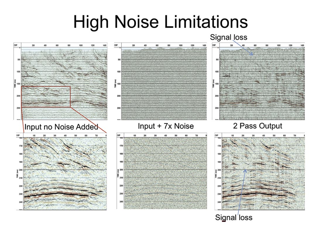
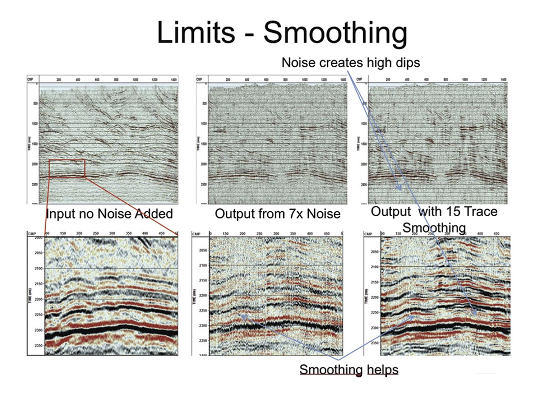
A stacked section which already contains some noise is combined with white noise band limited to match the data. The RMS level of this noise is about 7x the amplitudes on the strongest events on the section. I use 41 traces x 300msec. to create the basis functions. (about 6.4 x noise reduction). Signal is lost when the S/N ratio is about 30dB. (Figure 1) We are using two passes as three just makes the section noisier.

This result may be enhanced by applying smoothers to the amplitude and statics matches – shown in Figure 2. Note that the statics smoothers produce the typically wormy appearance of a mix. Even the strong events have a “jitter” due to the high amplitude noise. Notice that where the section is too noisy, high dip events are being created. This is actually an advantage as they can be easily seen and removed. If the programs were to create low dip events from the noise, these could easily be confused with signal.

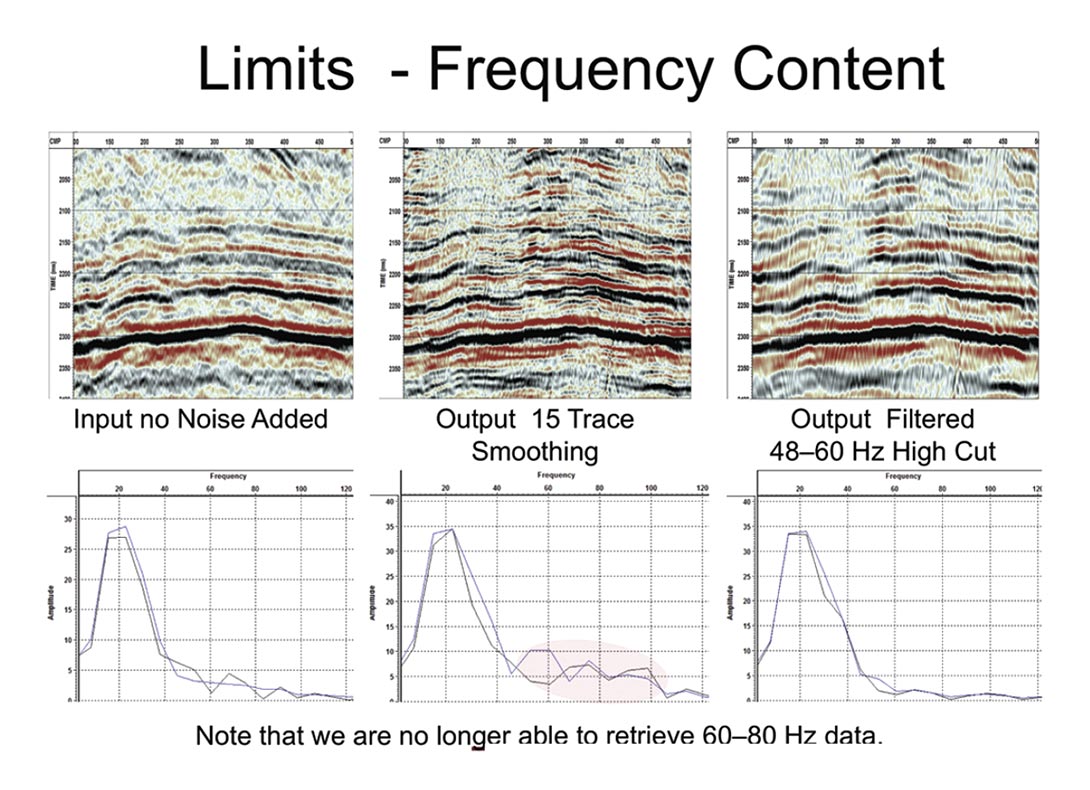
Zooming into this output for more detail we see that the smoothed events are higher frequency than the original input without added noise. This is a result of the statics we used ahead of the stacks used to create the basis functions. The statics have lined up noise and artificially whitened the wavelet. We can remove this by applying a 48-60 Hz high cut filter (Figure 3). This is a problem to be aware of (we are losing the 60-80 Hz data) but considering the section that we started with it is a small price to pay. Notice also that the diffraction patterns have been lost. This is a combination of the smoothers and the signal to noise.

Applications

Most of the signal can be extracted – even when it is badly contaminated with white noise. Here are some possible applications.

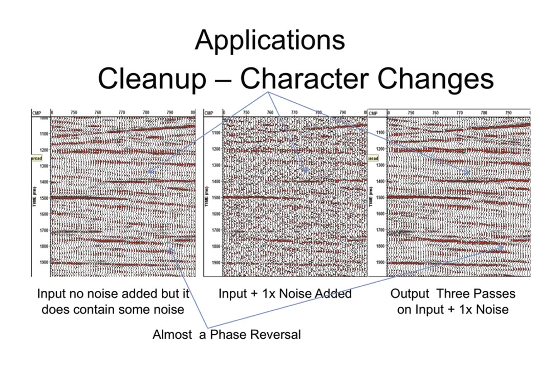
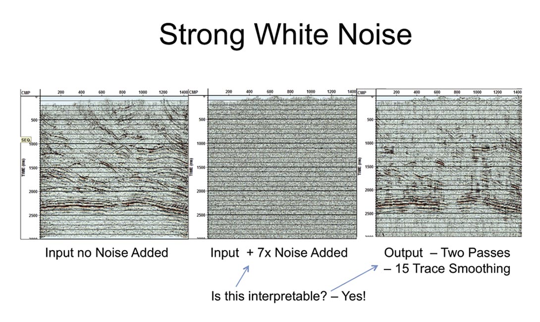
We can clean up the section (see Figure 4) and improve our ability to interpret it but pre-stack migration most of the time is a good noise suppressor too. If the pre-stack is noisy this program preserves sharp truncations and amplitudes and can be run on that too. Notice the phase reversal – it may also be run on gather data sorted by offset to enhance AVO. In Figure 5 if the section looks like the middle panel some analyzable data may still be recovered.

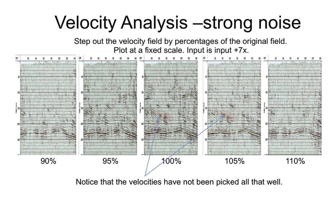
Because the algorithm preserves the original signal amplitudes we can NMO and stack with different percentages of the velocity field and pick velocities in movie mode. The amplitudes on the result (Figure 6) match the amplitudes on the input data so we preserve amplitudes section to section and can see which percent step-outs are brightest and most coherent. Notice that the original velocity picking was poor at the area highlighted. It should have been 5% faster.

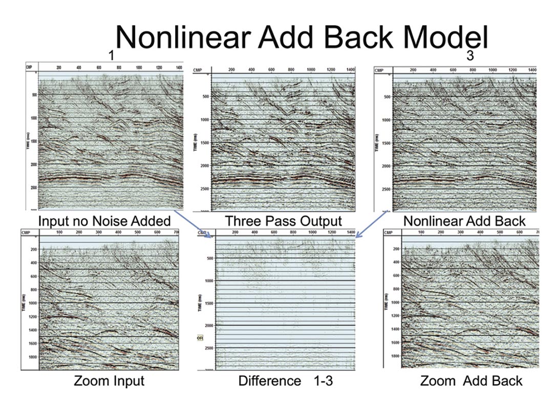
In Figure 7 you can see how we may also use these programs to enhance just particular areas on our section. We can clean up the section but where the data was noisy often the signal is still weak. If we can assume that the scalars are being affected by the higher noise in these areas, then it makes sense to add back the model nonlinearly into the original section bringing these areas to a minimum signal to noise ratio and adjusting the total amplitude to match the original amplitude. As you can see on the difference plot places where the signal to noise ratio exceeds the minimum are left untouched. Areas where the signal was weak are now normal and migration cancellation should be improved.

Finally we can use this process to whiten the wavelet on our section. If the noise is not too extreme the algorithm can extract most of the signal with the high frequencies intact. This process can be used before say spectral balancing is applied to flatten the high frequencies. Since the white noise is reduced, spectral balancing will work harder and the result will be a broader flat spectrum. Note that the old chestnut FXDECON and many other frequency domain programs cannot do this because they are unable to determine dips with the little signal we have at the high frequencies.

Unfortunately the phase of the high frequency data is unlikely to be correct. There is both DECON (the high end is way below noise) and NMO stretch to consider.

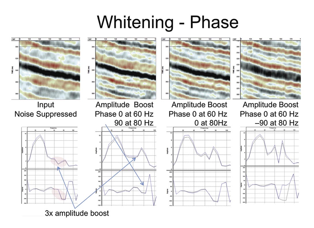
This has been analyzed by applying the algorithm and looking at the phase spectra of a number of events on the section – one of these events is shown in Figure 8. To flatten the spectra a phase ramp of 0 degrees up to 60Hz rising to 90 degrees at 80Hz has been applied to the whole section. Obviously it is not totally correct everywhere but it hopefully brings the phase into a range where it will stack. The original 100 degrees does not. Notice that on the section with zero phase shift the whitening has not really helped the resolution while the section with the phase shift is sharper and has not really changed the original event. To broaden the spectrum one must adjust the phase of the data being boosted.

Thus to whiten the data these steps should be followed – as shown in Figure 9:

• Remove the white noise with 4d,5dDEC and measure the phase on selected events.
• Phase correct the high frequencies in the original data.
• Apply the white noise removal algorithm.
• Subtract the white noise from the phase corrected data.
• Apply Spectral balancing.
• Add back the noise if desired.

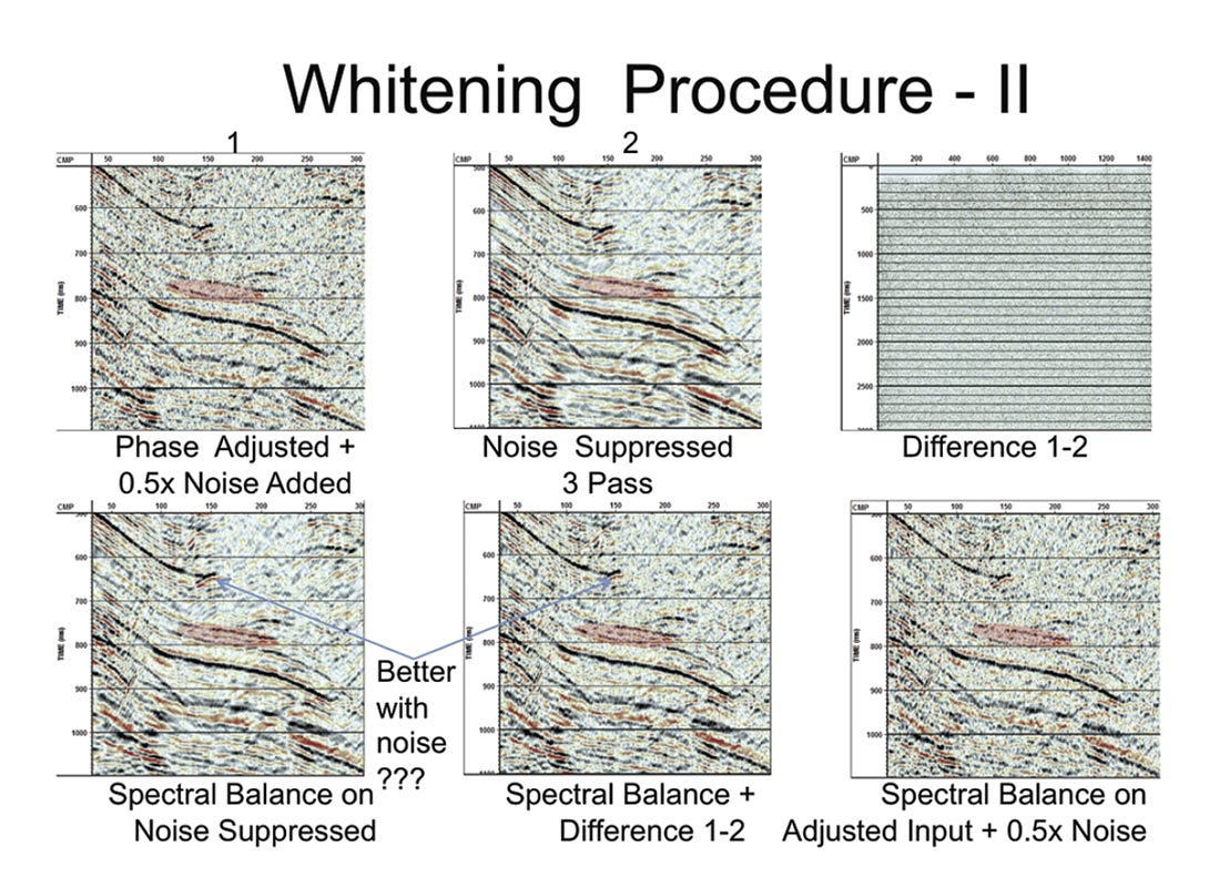
Notice that, as promised, the spectral balance with the white noise removal algorithm has worked a lot harder than just spectral balance on the phase adjusted input. Also the plain spectral balance fooled by the extra noise has not boosted the signal enough and has over boosted the noise in the input.

Conclusions Part II

White noise on seismic data does form the limit to our resolution. However by taking advantage of the local coherency in time and space of seismic data we have shown that we can make very large and valuable improvements to our sections. It has been shown that the algorithm can retrieve signal in the time domain even when the signal to noise ratio approaches 30dB. It can be used for velocity analysis, section cleanup and enhancement and spectral whitening.

In practice, the time domain principal component decomposition has proven to be a robust and effective technology. Almost the entire signal is preserved and only a few principal components at any time and place are needed.

If you respect that seismic data “wobbles” in space and time and changes in amplitude, then the seismic signal may be extracted relatively easily.

Acknowledgements

Thanks to WesternGeco for allowing me to present this material – Modules 4d,5dDEC from the seismic processing package VISTA from GEDCO at WesternGeco.