Summary
Wave equation migration (WEM) has been used in our industry for several years. Its ability to handle multiple arrivals from a surface position to a subsurface point provides us with higher quality images than Kirchhoff migration. However, apart from computational efficiency, WEM lacks some other advantages of Kirchhoff migration such as flexibility and the option to output image gathers in offset domain. In this paper, we present a migration approach based on summation of all contributions of individual traces to the image. This individual trace contribution is computed in the frequency domain by multiplication of the input data from a single trace and the Green’s functions with respect to source and receiver. Green’s functions are calculated through wave field extrapolation. The approach can be applied to both prestack depth and time migration and has all advantages of WEM as well as most of the advantages of Kirchhoff migration.
Introduction
Kirchhoff depth migration has been widely used in industry in the past decades due to its advantages of run-time efficiency, steep dip accuracy, flexibility and capability to output image gathers in offset domain. However, despite various high quality travel time computation techniques, Kirchhoff migration still has difficulty handling multiple arrivals. On the other hand, WEM automatically involves multiple arrivals through downward continuation of wave fields. We naturally seek a migration approach which is able to handle multiple arrivals and has most of the advantages of Kirchhoff migration.
The basis of Kirchhoff migration is the summation of all individual trace contributions. This allows any subset of the input data to be migrated to the desired imaging area. The individual trace contribution can be indexed with offset and this generates image gathers in offset domain after summation so that MVA in offset domain and AVO analysis can be performed. Also, regular spatial sampling is not necessary.
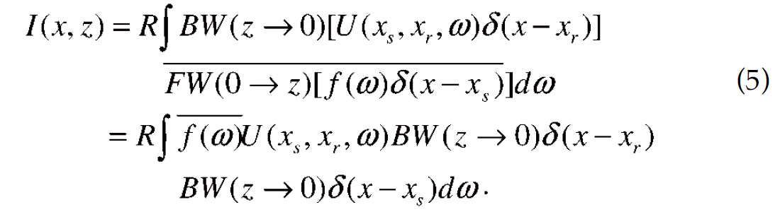
The approach in this paper calculates the individual trace contribution in the frequency-space domain by implementing Green’s functions at source and receiver positions. Green’s functions are computed by wave field extrapolation. The summation over all individual trace contributions and all frequencies forms the final image. We call this migration approach WESUM (Wave Equation Summation). This approach preserves all advantages of WEM and has most of the advantages of Kirchhoff migration. The procedure contains three steps, extrapolation, imaging and summation. The imaging step is much more expensive than the one in standard shot profile WEM, where it is negligible with respect to the extrapolation cost. However, proper wave field interpolation for Green’s function can greatly reduce the cost of extrapolation with little impact on image quality and the input of common shot gathers can make the imaging step computationally cheaper.
Description of the approach
For the sake of simplicity, we describe the approach through the convolution imaging principle

where P(x,z,ω) is the subsurface receiver wavelet, D(xs,x,z,ω) is the subsurface source wavelet and R is the real part operator. On the surface, P(x, 0, ω) is the recorded data and

with source spectrum f(ω). Assume P(x, 0, ω) is single trace with source position (xs , 0) and receiver position (xr , 0) and denote its value by U(xs ,xr ,ω), then

We denote the forward wave field extrapolator by FW( 0→ z) and then the inverse wave field extrapolator BW( z→ 0) equals to the complex conjugate of forward extrapolator (Ehinger, et al., 1996), i.e.

Thinking of D(xs,x,z,ω) as being extrapolated from the surface point (xs ,0) to subsurface point (x,z) and P(x, z, ω) as being extrapolated from (x,z) to (xr ,0) and considering linearity of extrapolator, we can rewrite (1) as
We define Green’s function at the surface point a for inverse extrapolation as

Then formula (5) becomes
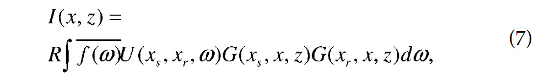
which can be referred to as the individual trace contribution formula.
To apply the formula (7) for prestack depth migration, we need to calculate Green’s functions for all source and receiver positions. In most of seismic acquisitions, the same surface position is reoccupied by many receivers and thus a given Green’s function can be used to calculate many individual trace contributions. In practice, we usually calculate reference Green’s functions at a certain number of surface locations and use spatial interpolation to obtain Green’s function at any source and receiver position. The wave field extrapolator is with respect to one-way wave equation and could be any type of extrapolation in frequency domain such as finite difference and PSPI (Phase Shift Plus Interpolation).
Since formula (7) is based on the individual trace contribution, the computation of which involves wave field extrapolation, it naturally handles multiple arrivals. The image can be indexed by offset and the migration is target-oriented and allows irregular spatial sampling. Theoretically, this approach is equivalent to standard shot profile migration.
Reduction of computational cost
The implementation of this approach needs three steps, extrapolation, imaging and summation. The imaging step is much more expensive than standard shot profile migration and is directly related to the number of input traces. To make the approach computationally more feasible, we try to reduce computational cost from both the extrapolation and the imaging steps.
We decrease the number of extrapolated Green’s functions by increasing the spatial interval of extrapolated Green’s function location on the surface when lateral velocity variation is not severe. In addition, we can increase the extrapolation step size and use some interpolation technique to obtain Green’s function at each depth level in image. Similar steps are done for travel time in Kirchhoff migration. The extrapolation step size has to be carefully selected to avoid aliasing and maintain accuracy.
The input dataset for this migration approach can be any type of gathers. However, there is potential for common shot gathers to have lower computational cost during imaging. For all traces belonging to one offset bin in a single shot gather, we perform multiplication between trace values and receiver Green’s functions, sum them and then multiply by the source Green’s function. This can be shown from the formula of one shot gather image
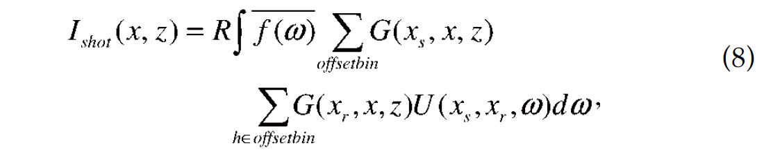
where h is offset with respect to source-receiver pair (xs , xr ). Compared with formula

for imaging one shot gather based on (7), the formula (8) has less complex multiplications.
Application to prestack time migration
The formula (7) is also valid for PSTM by substituting time t for depth z. For convenience we still use formula (7) in the following PSTM discussion. Unlike for PSDM, reference Green’s functions for PSTM are not with respect to surface locations but constant velocities. Assume the migration aperture is a, then we compute the Green’s function for a specific velocity value ν through

where BWv(t→ 0) is the inverse phase-shift extrapolator with respect to the constant velocity v. For any image point (x, t) with | x – xr | <a, and | x – xs | <a, we choose ν = vrfms(x,t), then the receiver Green’s function is obtained through

Similarly the source Green’s function is expressed as

The formulas (9) and (10) indicate that once the Green’s function at one image point is computed, it can be used to get all source and receiver Green’s functions needed for the image at this point.
Computing the Green’s function for each velocity value by using wavefield extrapolation is very expensive. Instead, we only perform wavefield extrapolation for a few velocities and then use interpolation to obtain all needed Green’s functions. The practical calculation can be described as follows.
1. Select the initial group of reference velocities

such that v0 and vn are minimum and maximum values of all velocities respectively.
2. After the time level i-1 is imaged, the minimum and maximum values of all velocities below the time level i-1 might be vl and vm (0≤l≤m≤n) . Apply the phase-shift extrapolation with the velocity vk (l≤k≤m) to the reference Green’s function Gvk (x,ti-1) to obtain the new Green’s function Gvk (x,ti-1). The new group of reference Green’s functions is generated at the time level i as the integer k scans from l to m.
3. If l=m, no interpolation is needed since the velocity field for remaining time levels is constant. Otherwise, for any image point P on the time level i with rms velocity v between vk-1 and vk (l+1≤k≤m) , calculate the Green’s function Gvk (x, ti) through the interpolation of functions Gvk–1 (x,ti) and Gvk (x,ti).
4. Obtain source and receiver Green’s functions for each sourcereceiver pair through (9) and (10), then get the image at all points within the migration aperture using the formula (1). The single-trace-contribution is thus calculated.
5. Sum all one-trace-contributions for all source-receiver pairs to get the image at time level i and then return to step 2 to image the time level i+1.
Step 2 and Step 3 are PSPI procedures and the fourth step is actually an imaging process. Unlike the method of Ekren and Ursin (1999), the extrapolation is recursive and the group of reference velocities covers not only one single time level but all time levels that need imaging. The number of reference Green’s functions decreases with the downward migration because the velocity range usually becomes smaller and smaller. The main computational cost is spent in step 4 where the number of complex multiplications is proportional to the number of frequencies and to the size of the image volume.
WESUM PSTM for land data
Most 2D land datasets are not straight profiles and many are with rugged topography. These are very challenging for the usual WEM application.
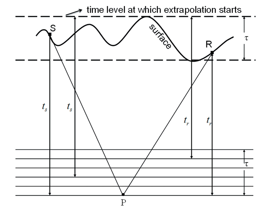
Migration geometry from topography requires the extrapolation to be started from source or receiver position, usually not at the top time level. For those reference velocities which will be used for imaging, we store their reference Green’s functions for a few time levels in memory or disk. The number of these time levels is the same as the one that the recording surface occupies. In Figure 1, this number is six. Of these six time levels, the lowest one needs imaging. Assume the rms velocity at the point P is v and its nearest reference velocities are v1 and v2. For each of these two velocities, the Green’s function is selected from its six stored reference Green’s functions for calculating source Green’s function through the interpolation. The extrapolation for this selected Green’s function should pass through the same number of time levels as between source position and the imaging time level so that it could be equal to the Green’s function whose extrapolation is from the source position to the imaging time level. In Figure 1, let ![]() and
and ![]() (l≤i≤6) denote reference Green’s functions for v1 and v2 at the ith time level of the six. Then Green’s functions
(l≤i≤6) denote reference Green’s functions for v1 and v2 at the ith time level of the six. Then Green’s functions ![]() and
and ![]() are selected to generate the source Green’s function through the interpolation and similarly the interpolation of
are selected to generate the source Green’s function through the interpolation and similarly the interpolation of ![]() and
and ![]() generates the receiver Green’s function.
generates the receiver Green’s function.
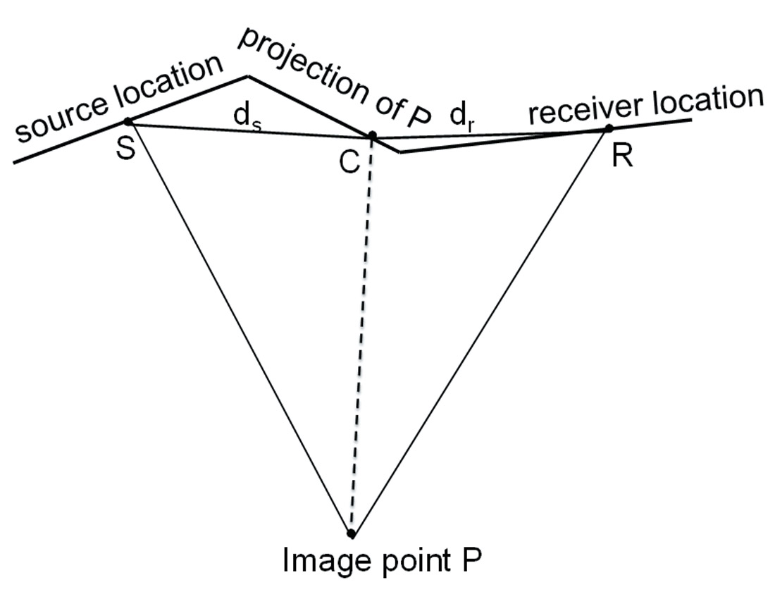
Migration geometry for the 2D crooked line can be illustrated in Figure 2, where S and R are source and receiver locations and C is the projection of the image point P to the surface. Let ds denote the distance from the point S to the point C and dr denote the distance from the point R to C. These distances can be used to calculate source and receiver Green’s functions through replacing x-xr and x-xs in (9) and (10) by a-dr and a+ds respectively. The sign for ds and dr depends on if the source (or receiver) location is on the left or right side of the point C. Here we assume the source is on the left side and the receiver is on the right side. In this way, there is no need for source, receiver locations and the surface point C to be on the same straight line and hence the 2D crooked line geometry is handled.
Data examples for PSDM
Figure 3 compares the performance of WESUM algorithm on the Marmousi synthetic data. Figure 3a shows a line segment with standard shot profile WEM migration and Figure 3b shows the equivalent WESUM display.
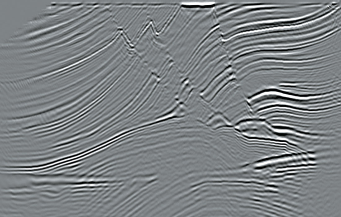
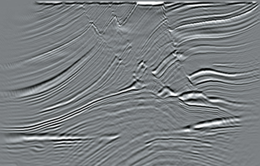
The data examples show that images from WESUM are comparable with standard shot profile migration. All extrapolation tools are PSPI which can tolerate large extrapolation step size.
Data examples of PSTM
Figure 4 and Figure 5 show more example comparisons of WESUM and Kirchhoff migration for PSTM for both European and Alberta foothills data.. One can notice in the highlighted areas that WESUM has handled the steep dips better than Kirchhoff.
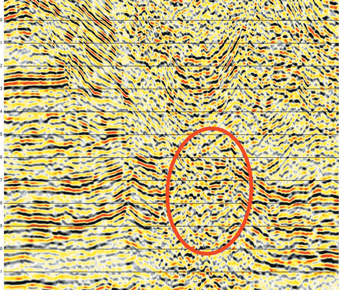
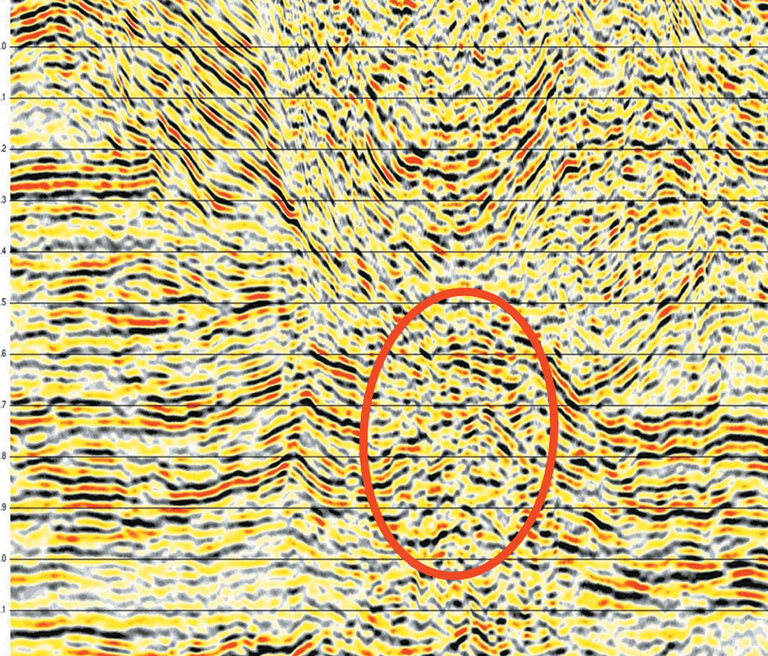
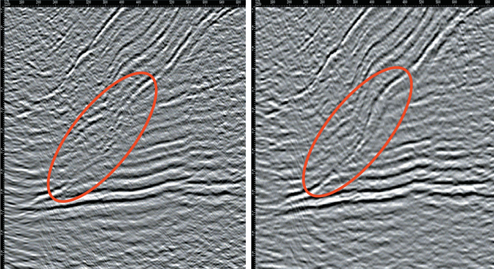
Figure 5b. Alberta foothills image from WESUM PSTM (right).
Conclusion
We have presented a new migration approach based on summation of individual trace contributions combined with wave field extrapolation. The approach can handle multiple arrivals for depth migration and also perform targeted migration. The image gathers could be offset-indexed. In the application of prestack time migration, wave field extrapolation with constant velocity is performed to calculate individual trace contribution. Data examples from synthetic and real seismic data show the comparison of WESUM images with standard shot profile WEM images in PSDM and also with Kirchhoff images in PSTM.

Acknowledgements
We wish to thank Arcis Corporation for encouraging the development of this work and for permission to publish it.


Join the Conversation
Interested in starting, or contributing to a conversation about an article or issue of the RECORDER? Join our CSEG LinkedIn Group.
Share This Article