VSP Reflection Points for Linear Inhomogeneity and Elliptical Anisotropy

Abstract

An exact analytical expression for traveltime in a medium with a constant velocity gradient and elliptical velocity dependence is used to calculate possible reflection points for a given source receiver geometry. The set of reflection points are collectively referred to as the illumination zone. Also, we give an expression that can be used to trace rays in a vertically inhomogeneous elliptically anisotropic medium. These expressions are applicable for both survey design and data interpretation.

Introduction

Under certain simplifying assumptions, which often appear to be reasonable in exploration seismology, there exists a convenient analytical expression that gives the traveltime of a signal as a function of the source and receiver positions. We will use this equation to determine the zone of all possible reflection points for an offset VSP, as well as to trace trajectories of the signal. In the remainder of this paper, we will refer to the collection of reflection points as the illumination zone and to the trajectories as rays.

The aforementioned assumptions, which are required to derive the traveltime expression, are lateral homogeneity, which is commonly associated with the study of sedimentary layers, and elliptical anisotropy, which allows us to consider directional dependence of velocity encountered in such layers. These assumptions are commonly made when modeling an equivalent medium that allows us to account for the observed traveltime. We begin by describing the traveltime expression.

In this study, we consider a two-dimensional case where we use the xz-coordinate system with x and z corresponding to the horizontal and vertical axes, respectively. Throughout this paper, we set the origin of this system to be located at the source. We assume that the properties of the medium are laterally homogeneous. That is, the properties vary only with depth, z. Furthermore, we assume the magnitude of ray velocity increases linearly with depth and that the directional dependence is elliptical. In such a case, the ray-velocity expression is

(e.g., Monagan and Slawinski, 1999). Parameters a and b describe the linear increase of velocity with depth, which may be due, for example, to increasing compaction. θ is the ray angle, which is measured from the z-axis. It is assumed that the ellipticity is constant and given by

where V_x and V_z are the horizontal and vertical ray velocities, respectively. We refer to the medium described by equations (1) and (2) as the abχ model.

Direct-arrival traveltime between the source at (0,0) and a point at (x,z) in a medium described by a ray-velocity stated in expression (1) is

where

(e.g., Slawinski, et al., 2003). In the case of isotropy, where χ=0, expression (3) reduces to that of Slotnick (1959). Parameter p is the conserved quantity along the ray for a given source-receiver offset and is commonly referred to as the ray parameter.

Having stated expression (3), we can now illustrate its application in determining the illumination zone. This method, for instance, would allow one to investigate the source-receiver geometry necessary for imaging a particular area of interest in the subsurface.

Method and Results

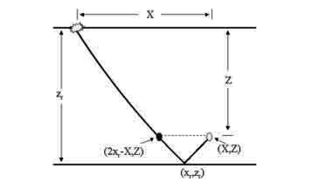
Given the borehole-receiver location, (X,Z), and an interface depth, z_r, we wish to determine the location of the reflection point, (x_z , z_r). Having analytical traveltime expressions, we can achieve this by invoking the principle of stationary traveltime. Since lateral homogeneity implies horizontal interfaces, it could be shown that the signal propagates along the least-time trajectory, which is the ray.

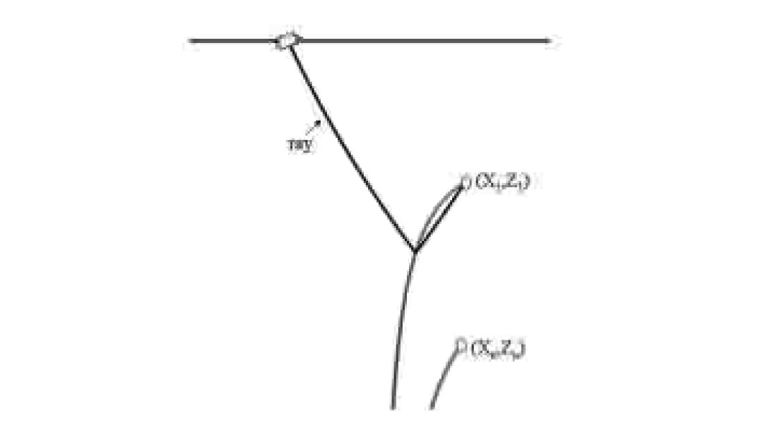
In view of lateral homogeneity, the ray is symmetric about the vertical line passing through the reflection point. Hence, for a given receiver at (X,Z) we can write the traveltime of the reflected signal as

Examining Figure 1, we see that the first term on the righthand side is twice the traveltime from the source to the reflection point. The second term on the right-hand side is the traveltime along the ray from the source to the depth that is equal to the receiver depth.

For a given interface, using expressions (3) and (5), we can explicitly write the traveltime expression for a reflected signal between the source and a given receiver. To find the value of x_r, corresponding to the stationarity of traveltime, stated by expression (5), we use numerical methods. Our code is shown in Appendix A.

By determining x_r for various interface depths, we can trace the set of possible reflection points for a given receiver position, (X,Z). If we perform this process for both the shallowest and the deepest receivers, we generate the two sets of reflection points shown in Figure 2. The zone bounded by these two curves and by the wellbore containing the receivers represents the illumination zone for the given source and set of receivers.

In general, to obtain the illumination zone, we must resort to numerical methods to find x_r . To illustrate the case where we can obtain a closed-form expression for the reflection point in terms of receiver location and reflection depth, consider the case of homogeneity (i.e., b=0). In principle, solving for the reflection point in a homogeneous medium, involves finding the limit of expression (3) as b tends to zero, then finding the stationary point of the resulting reflected traveltime expression, as shown in Appendix B. However, below, using the fact that rays in homogeneous media are always straight, in order to illustrate our general approach, we will follow the method analogous to the one used above.

Using the Pythagorean theorem, we get the reflected traveltime as

where V₁ and V₂ are the velocities of the downgoing and upgoing signals, respectively. Expression (6) contains the information that, for the general case, is given by expressions (3), (4) and (5). To find explicit expressions for V₁ and V₂ , we use expression (1) with the ray angles expressed in terms of the reflection-point and the receiver-location coordinates. Thus, we obtain

and

Inserting expressions (7) and (8) into expression (6), we can explicitly write the traveltime expression for a reflected signal between the source and a given receiver in a homogeneous medium. Now, we can invoke the principle of stationary traveltime. Setting the derivative of expression (6) – where V₁ and V₂ are given by expressions (7) and (8), respectively - with respect to xr to zero and solving for x_r, we obtain

The algorithm that uses expression (9) is shown in Appendix C.

We note that in deriving expression (9) we assumed the medium to be homogeneous and elliptically anisotropic. However, since χ disappears in the process of differentiation, expression (9) is equally valid for both isotropic and anisotropic homogeneous media. As stated above, this is a result of the fact that in homogeneous media all rays are straight. In other words, in homogeneous media, anisotropy does not affect the rays. It does, however, affect the traveltime of the signal along these rays.

Discussion and Conclusions

Given the values of parameters for an abχ model, we can determine the illumination zone for a given source and a set of receivers. In particular, our results allow us to obtain — for a given source-receiver pair — the location of the reflection point at a given depth. To see the importance of this relation, consider the following example.

Dividing both the numerator and denominator of the right-hand side of equation (9) by z_r and letting z_r tend to infinity, we see that for very large depths, the reflection point is approximated by the midpoint between the source and the receiver. In the context of seismic exploration, however, expression x_r≈X/2 applies to depths that are beyond those of exploration interest. For most cases of interest, reflection points tend to be significantly closer to the receiver than to the source. To illustrate this point, consider an abχ model, where a=2000m/s, b=0.8s^-1 and χ=0.3 which are reasonable values for the Western-Canada Basin. (We note that these values were also used to plot both Figure 1 and Figure 2). Let the receiver be located at (1000m,1000m). For an interface at a depth of 2000m, the reflection point is located at (635m,2000m) — a significant distance from the midpoint.

Expression (4) has another convenient application that was also used in this paper. Knowing the reflection point we can obtain the closed-form expression that can be used to trace the ray. This is achieved by solving expression (4) for x to get

To find the value of p, simply substitute any point along the ray (e.g., the reflection point) that corresponds to a given source receiver pair, into expression (4). The rays shown in Figures (1) and (2) are traced using expression (10).

We note that our formulation can be used in deviated wells since all equations require only the relative location of a given source and a given receiver. In other words, these equations are associated with point-to-point problems. In all cases, the illumination zone is bounded by the upper and lower curves that correspond to the refraction points and by the wellbore.

As stated in the introduction, given a set of observed traveltimes we assume an equivalent medium given by the abχ model and determine the values of a, b and χ to account for the observed traveltimes. In interpreting VSP data we must bear in mind that given a source-receiver position and a traveltime there exist an infinite number of velocity fields and an infinite number of rays that will give the observed traveltime. In particular, if there are localized regions between the source and the receiver in which the velocity differs greatly from the model this will affect the rays and hence the reflection points. Consequently, even though an abχ model is a reasonable approximation, we expect local discrepancies between the computed reflection points and field results.

Acknowledgements

We would like to acknowledge the constructive comments of David Dalton and the valuable editorial work of Cathy Beveridge. As this study has been done in the context of The Geomechanics Project, the authors wish to acknowledge the Project sponsors: EnCana Energy, Husky Energy, and Talisman Energy.