Using Multi-Well Microseismicity to Identify Fracture Types Associated with Hydraulic Fracture Stimulations

Abstract

BP deployed microseismic monitoring arrays in two observation wells in a Rocky Mountain tight gas province for the purpose of mapping hydraulic fractures in a nearby lateral. Engineering Seismology Group (ESG) collaborated with BP to conduct an advanced re-analysis of the large data set obtained from the dual-well microseismic monitoring program. The goals of the re-analysis included recalculating observed fracture azimuths and selecting a subset of events with good signal-to-noise ratios and key signal characteristics (e.g., distinct P- and S-wave first arrivals, amplitude data and first motion polarities) to conduct further, detailed analyses. Event locations were recalculated, combined with signal characteristics and inverted to solve for moment tensor solutions. The derived set of solutions provides a robust determination of fracture azimuth as well as offering additional, unique insights into the stress history in the vicinity of the project. As such, these more comprehensive, in-depth microseismic analytical techniques have proven themselves to be valuable tools that can increase understanding of local geology and stress histories, thus aiding design of effective, future fracture treatments.

Project Background

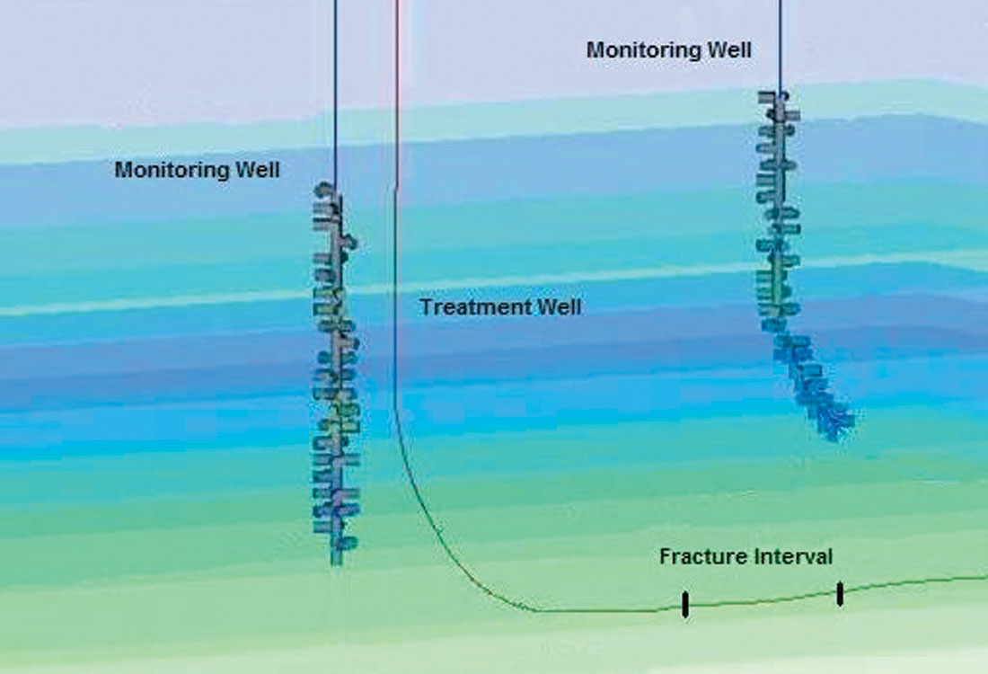
Two microseismic monitoring arrays were deployed, one array in each of two relatively vertical wells spaced less than 1500 meters apart, near a third lateral well that was subsequently hydraulically fractured (Figure 1). The arrays deployed in each of the monitoring wells consisted of 22 triaxial geophone levels, each spaced about 15 meters apart, with the deepest level set approximately 70 meters above the zone being stimulated in the adjacent lateral. The project area is located in a Rocky Mountain tight gas province. Formations in the project area are of Mesozoic age, nearly flat-lying and consist of clastic sediments.

During the subsequent fracture treatment, a large data set was recorded from which ESG manually extracted 81 events that were judged to have acceptable first motion (P-wave) arrivals and high signal-to-noise ratios. Selection of the 81 best-quality events involved first conducting an automated and summary manual review of the entire microseismic monitoring data set, then conducting a more detailed manual review of a total of 15,552 waveforms – one waveform for each X, Y and Z axis for each geophone level – to determine the quality of first arrival picks.

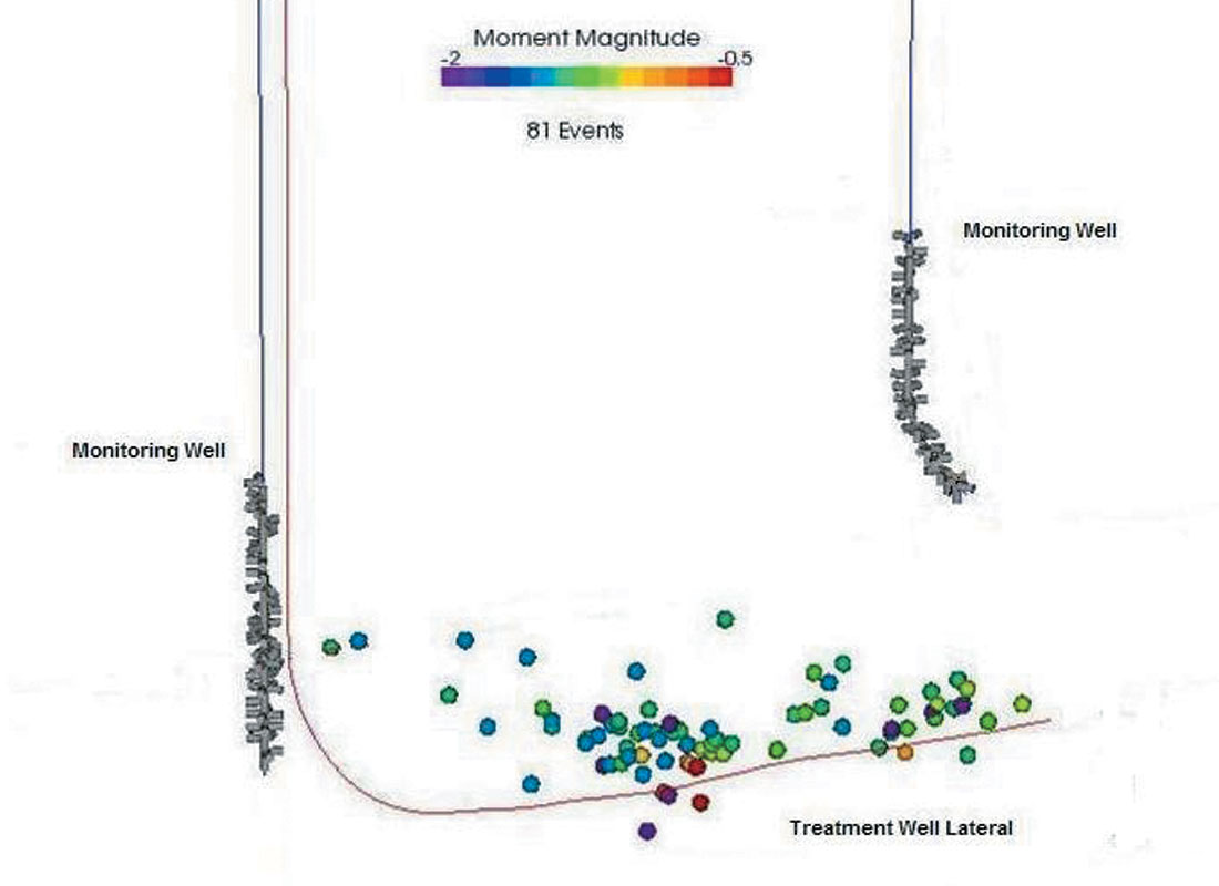
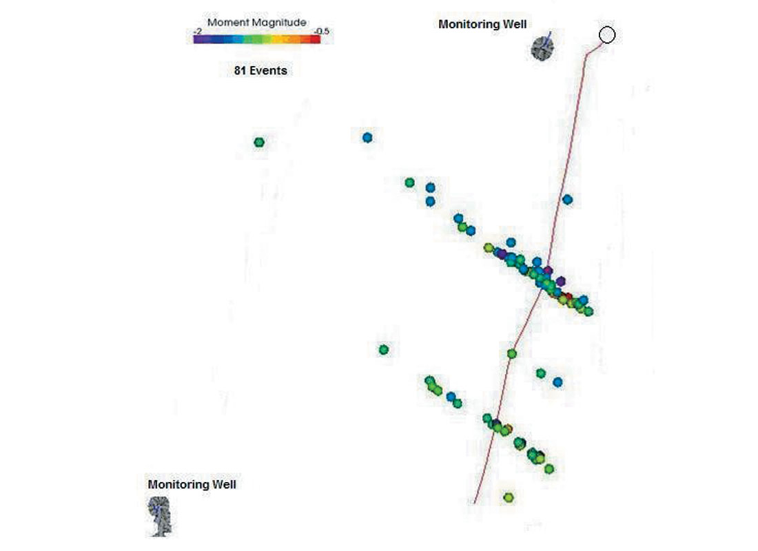
A total of 5,568 rotated waveforms were analyzed to determine first motion. Event threshold parameters were set to include a minimum of five channel triggers and a twice-background signal-to-noise ratio; 200 milliseconds (ms) time windows were used to isolate waveforms. The events studied were limited to only those that registered on both sensor arrays and had a high signal-to-noise ratio. After further processing and data evaluation that emphasized the quality of orientation results, signal-to-noise ratio and quality of signal, a subset of 29 events met the criteria and were inverted for failure characteristics (Figures 2a and 2b).

Adjustment of Velocity Model Based on Sonic Log Information

Initially, waveforms from a single string shot, conducted prior to the hydraulic fracture treatment in the lateral, were used to orient and calibrate the sensors. However, when the orientation calculated using this string shot was applied, inconsistencies and discrepancies were observed between the known location and that derived by the inversion of first arrival data. To improve the solution for the string shot and associated seismic data, ESG reevaluated the original velocity model provided by BP. In the original velocity model, P-wave velocities were observed to be significantly lower than the average value derived from a dipole sonic log collected from a nearby well. An attempt was made to resolve the observed log-model discrepancy by modifying the velocity model, which was expected to improve the calculated solutions for the string shot relative to the orientation of the sensor arrays.

In conducting its re-evaluation, ESG kept the original model layers intact and two different velocity models were derived using these layers:

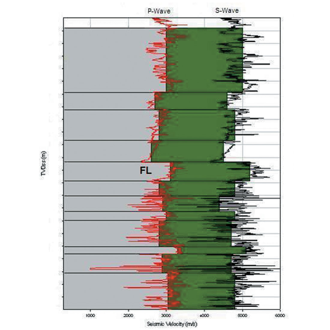
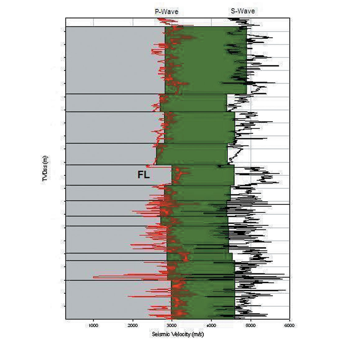
• Initial Velocity Model. ESG created its own in-house velocity model (Figure 3) based on the same dipole sonic log used to create the original velocity model. ESG determined that the derived average velocities were generally much higher than those associated with the original velocity model provided by BP. A large part of the effect was based on one particularly “fast” layer (marked as “FL” on Figure 3) that changed most of the subsequent algorithms substantially.
• Second Velocity Model. Employing an inversion program to force the location of the calibration string shot, ESG made a second attempt to develop a workable velocity model. Although this approach gave the best result when locating the string shot, it resulted in large residual misfits between the actual and theoretical P- and S-wave arrivals.

Without further detailed information on the site, including well geometries and formation tops in the observation wells, the original velocity model was deployed in the event location algorithms (Figure 4). Based on this velocity model, locations were calculated for the selected subset of events. In spite of the issues identified, locations were obtained. However, the unresolved velocity issues added to the location uncertainty in the final results.

Wave Form and SMT Analysis

The original waveforms were rotated into their raypath directions using a hodogram analysis, resulting in waveforms oriented in P, Sv (vertical) and Sh (horizontal) directions. From these rotated signals, P- and S-wave arrivals were selected as well as P, Sv and Sh polarities and amplitudes for each sensor. A subset of 29 events with well-defined P, Sv and Sh waveforms were inverted using a modified version of the simultaneous moment tensor (SMT) inversion algorithm developed by Trifu and Shumila (2003) that accounts for a layered velocity model.

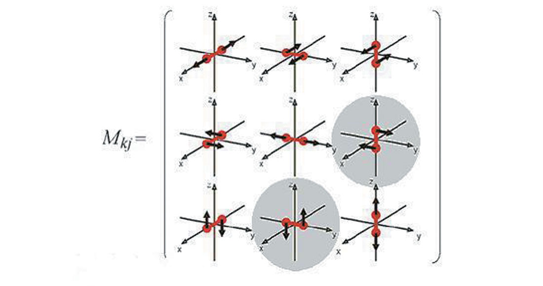
When conducting an SMT analysis, solutions for six unknown moment tensor components (Figure 5) are being sought. If only deviatoric (zero-trace) tensors are considered, the number of unknown parameters is five. Inversion quality is estimated through the Condition Number (CN), defined as the ratio between biggest and smallest eigen value of inversion matrix for the volume of interest, and by means of Monte-Carlo simulation utilizing trial seismic source locations.

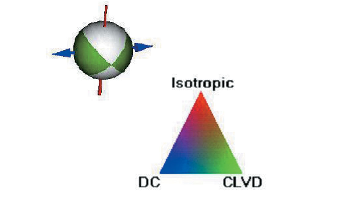
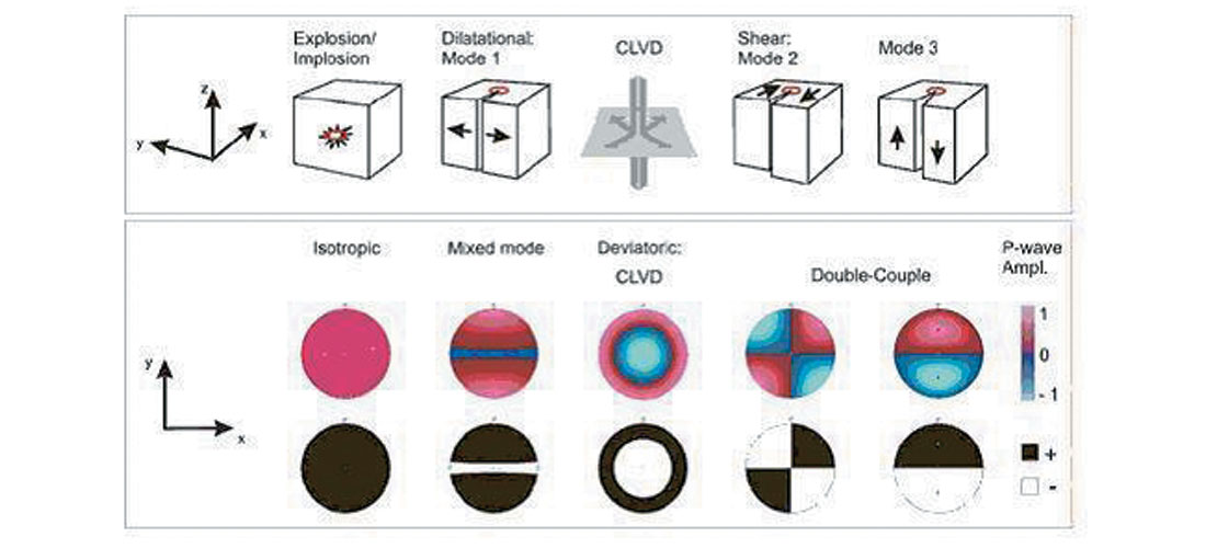
For the purposes of visualizing the SMT solutions, a traditional “beach-ball” form is used to illustrate the relative strain axes (P-, B-, and T-axes), failure planes, and the failure mechanisms themselves (Figure 6). The coefficients of the SMT solutions allow for the failure mechanism to be defined in terms of the double couple (DC), isotropic and CLVD (Compensated Linear Vector Dipole) components of the failure (Figure 7). Looking at the variability of solutions for distinct groups of events provides further insight into the general failure process within the volume affected by the hydraulic fracture treatment.

Results and Conclusions

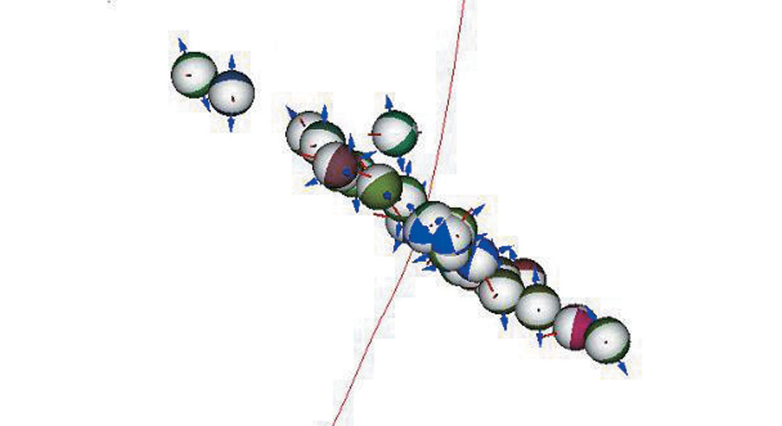
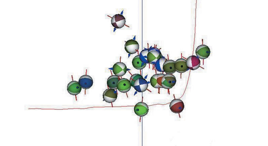
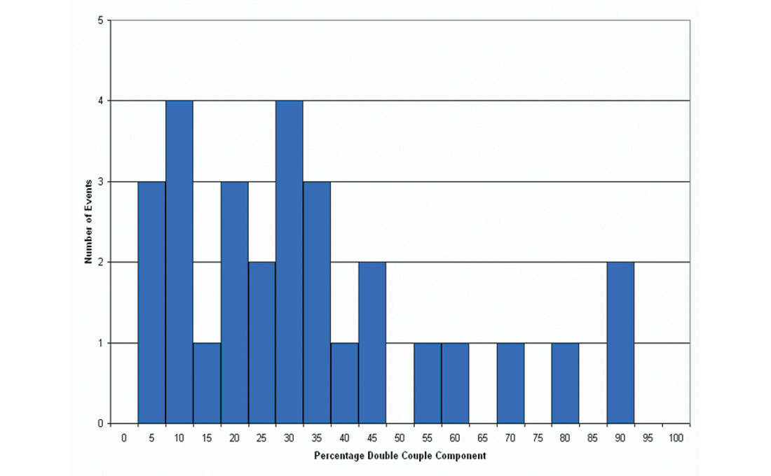
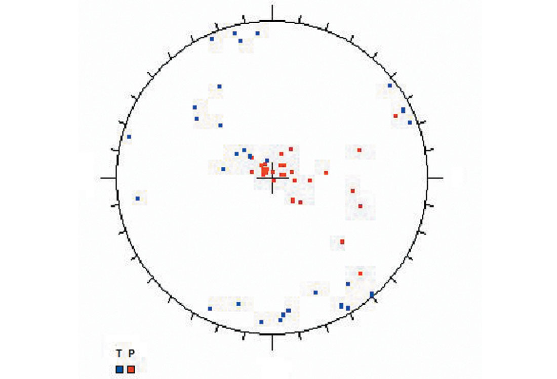
Selected views of the space distribution results for the SMT analysis are shown on Figures 8a and 8b. The majority of the SMT solutions derived for the 29 events have a double-couple (shearing) component of failure and most of the event failures appear to consist of a complex fracture process rather than a simple ‘fault-slip’ type mechanism (Figure 9). This information can be combined with a stereographic P- and T-axis plot (Figure 10), which indicates the P-axis (red) is sub-vertical for the majority of the events and the T-axis (blue) is more scattered, generally with a sub-horizontal orientation, suggesting a normal mode of failure.

Based on this study, it is evident that when multi-well recordings are available, additional information related to the stimulation process and the local fracturing conditions can be obtained by a closer examination of microseismicity. Making use of these data can provide operators with significant insights into how to optimize their hydraulic fracturing designs to potentially improve production.

Acknowledgements

ESG greatly appreciates the assistance of Jim Wolfe and BP in organizing and supporting the study discussed in this paper, and for permission to publish.