Tight Gas Geophysics: AVO Inversion for Reservoir Characterization

Summary

A general discussion of some of the critical steps in AVO inversion workflows is included with a Western Canadian case study in this paper. We use the case study to illustrate that the ratio of the compressional and shear wave velocities (Vp/Vs) is a useful indicator of quartz-clay ratios in log data, and by extension suggest that Vp/Vs data from AVO inversion provide a means of characterizing, at least qualitatively, reservoir properties.

The case study utilizes petrophysical data processed in a consistent manner to produce mineral volume logs over the Doig and Montney Formations in addition to micro-seismic monitoring data from a horizontal well stimulation. These data are qualitatively correlated to the AVO inversion data. This case study, then, represents at least part of an integrated workflow for reservoir characterization in tight gas and shale gas plays.

Introduction

Integrated workflows for shale gas reservoirs have received increased attention following the step changes achieved in operational efficiency over the last decade. Du et al. (2009) presented such a workflow for the Barnett Shale play in Texas; however, a crucial link missing in their workflow was analysis and inversion of pre-stack seismic data. In Western Canada an increasing number of major leaseholders in the Horn River Basin and operators exploiting unconventional reservoirs in the Montney Formation are utilising pre-stack amplitude variation with offset (AVO) inversion data to assist in well placement and field development planning. However, such data is typically regarded differently by different members of an asset or development team. As reservoir characterization workflows for shale gas plays evolve, geophysicists must stress the place of 3D seismic data and advanced products (such as AVO inversion) in the workflow and illustrate means by which the data can be integrated in a manner that brings maximum uplift and assists in understanding lateral heterogeneity.

AVO inversion of 3D seismic data allows for the creation of Vp/Vs (or Poisson’s ratio and/or lambda-mu-rho) volumes and maps of the reservoir interval, which reflect the heterogeneity of the reservoir associated with grain size and minerallogy. However, inversion data and other attributes derived from pre- or post-stack seismic data require corroboration from independent sources to confirm their utility. Data that can provide such calibration for these seismic based properties includes log based petrophysical data, micro-imaging data, production log data, production data, and microseismic monitoring data.

The heterogeneity of reservoir rocks within shale gas plays has been well established through wireline logging and coring and through empirical observations of stimulation and production response. Logging programs developed during the early part of this century to include spectroscopy based tools, which are capable of providing estimates of elemental proportions by weight and the relative abundance of naturally gamma-ray emitting elements (potassium – K, thorium – Th, and uranium – U). Determining elemental proportions allows the mineral contents to be determined and specifically the types of clay minerals present. Understanding the relative abundance of K-U-Th also assists in establishing total organic carbon (TOC) within the rock as kerogen can often be rich in Uranium. Shear sonic data and micro-image logs have also established their utility as they can identify changes in local stress associated with mineralogy, anisotropy in horizontal stress associated with tectonic forces, and natural fracture properties and abundance.

1. Petrophysical Data and Modelling

The area of Western Alberta where unconventional plays within the Montney and Lower Doig Formations are currently being exploited is mature in terms of exploration and production for conventional resources. Accordingly, there are a large number of wells that penetrate the Montney and Doig Formations that have been logged with standard triple-combo logging suites (i.e., resisitivity-density-neutron logs). In the absence of spectroscopy data in older wells it is necessary to carefully construct petrophysical models capable of predicting mineral contents and TOC from standard log curves.

Key reservoir parameters, including total and effective porosity, mineral volumes (clay, quartz, carbonate), and volumes of kerogen and TOC can be estimated from standard log data where robust petrophysical models can be created. In the following case study a petrophysical model based on basin wide studies in the Western Canadian Sedimentary Basin (WCSB) is utlilized. This model was constructed using classical statistical analysis techniques such as; histogram/frequency analyses, normality tests, cluster analysis and uncertainty analysis. Although such a model is no replacement for acquisition of high quality log data, in fields where there is little or no existing spectroscopy data and very little shear sonic and micro-image log data, empirical models that can accurately transform standard log data to advanced outputs are invaluable.

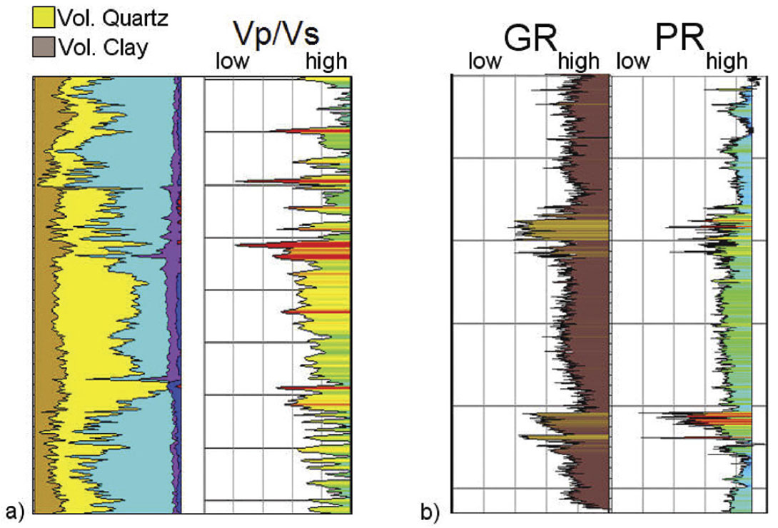
Where advanced logs and shear velocity data are available, the vertical heterogeneity through the potentially prospective zones can be measured. From these data it is observed that, in general, the ratio of compressional to shear sonic velocities (Vp/Vs) is a good indicator of sand-shale or quartz-clay ratios in shales and/or tight siltstones (Figure 1). Qualitatively and empirically, an increased sand-shale ratio correlates to increased porosity, lower breakdown pressures for stimulation, and enhanced relative production (Miller et al., 2007).

2. Amplitude Variation with Offset Inversion

AVO techniques exploit relative changes in seismic reflection amplitudes at varying incident angles to quantify changes in elastic properties at reflection boundaries, which can provide information regarding lithological and fluid properties of the formations. Through AVO inversion it is possible to derive an earth model that is consistent with measured seismic reflection data. This model can illuminate prospective subsurface areas characterized by anomalous physical properties (i.e., hydrocarbon reservoirs).

Seismic inversion techniques have been utilized since the 1970s (Pendrel, 2001). The implementation of inversion methods in the analysis of pre-stack seismic data (typically offset or angle stacks) provides the ability to derive quantitative estimates of the physical parameters that control the AVO response, namely the compressional and shear wave velocities and density, which can then be compared directly to measured well log data. Not only do the properties derived in the inversions have real physical meaning, they also benefit from the removal of wavelet effects and damping of noise outside the inversion operator range.

Standard AVO inversion workflows share a number of common steps; a brief discussion of some of the most critical (listed below) follows:

1. extracting wavelets,
2. low frequency modelling,
3. data inversion.

2.1. Extracting wavelets

The seismic wavelet represents the energy illuminating the subsurface and provides the connection between the subsurface elastic properties and seismic reflection data. This connection is represented through the convolutional model, which states that the seismic trace is the result of a convolution between a source wavelet and an earth reflectivity series. A typical wavelet extraction process uses the concept of the convolutional model where a wavelet can be estimated by solving an inverse problem when the seismic trace and reflectivity series (calculated from well logs) are known. Because a convolution is a stationary process, this automatically assumes stationarity of the wavelet within the extraction window. Therefore, inversions that incorporate a wavelet are typically target oriented to justify the stationary wavelet assumption. To further compensate for the non-stationarity, separate wavelets are estimated independently for each angle stack using an angle dependent reflectivity series. This allows for a better representation of the offset dependent amplitude and phase variations observed in seismic data. It is also possible to implement time-varying wavelets, in amplitude and frequency, in some seismic inversion workflows. A time-varying wavelet can be important where assumptions regarding wavelet stationarity are not necessarily valid (e.g., where long estimation windows are required).

As the sonic and density logs are measured in depth and our seismic data in time, it is necessary to establish a time-depth relationship to relate the two domains. Where checkshot data are available, velocities are typically well constrained. In the absence of checkshot data, however, it is common to use prior knowledge about seismic horizons from regional surveys and geological formation tops (interpreted from well log data) as a guide along with sonic velocities measured during logging. Sonic velocities may be misleading as rarely are sonic data recorded to surface and as the well logs are measured at higher frequencies, relative to surface seismic data, the sonic velocities can be up to 10% higher than reflection seismic velocities.

To compensate for mis-ties between log-based synthetic seismograms and reflection data it is often necessary to make manual adjustments to the synthetic. However, there is much debate about the validity of this ‘stretch-squeeze’ approach. Indeed, with no a priori information about the source signature, it is typically not possible to determine definitively the amplitude and phase of the extracted wavelets and predict the correct velocity profile using stretch-squeeze corrections. When only one well is available for wavelet extraction, this non-uniqueness is an intractable problem. However, where multiple wells can be used to test wavelets, it is generally possible to predict a wavelet that produces synthetics with strong correlation to the reflection seismic data at multiple well locations.

A common pitfall of wavelet extraction is the over-reliance on statistical measures of fit between synthetic seismograms and measured data. If, as most algorithms do, a least squares approach is taken to wavelet extraction, the extracted wavelet will incorporate noise in a relentless attempt by the least squares algorithm to minimize misfit at this singular location. Therefore, wavelets with many side-lobes will generally improve measures of cross-correlation locally, but it is wrong headed to assume that this will provide a representative wavelet for the entire survey as this approach is simply incorporating local noise in the seismic data and errors in the log data measurements.

2.3. Low frequency modelling

Due to the band limited nature of seismic data, a low frequency (typically below ~10 Hz) model (LFM) is needed to represent the true elastic properties and must be included in the inversion solution from sources other than seismic reflection data. This information is typically obtained from well log data where a low pass filter is applied to isolate the low frequencies required for the inversion solution. Interpolation methods are generally utilized to populate the LFM by extrapolating calibrated logs using interpreted horizons and faults. The low frequency model may also be constrained by seismic velocities, depth trends and dip fields estimated from the seismic data or observed stratigraphic relationships.

The most critical decision in constructing the LFM is the number of wells selected to influence or contribute. As the questions of where and how properties change relative to the well control points are unknown, constructing an LFM is inherently interpretive and non-unique. Therefore, proper care must be exercised in the interpretation of the low frequency trends in the final inversion property volumes.

2.4. Seismic Data inversion

The basis of all AVO studies is the plane wave Zoeppritz equations, which are parameterized in terms of P-wave velocity (Vp), S-wave velocity (Vs) and density. However, due to its complex nature, approximations were sought to obtain a more practical representation of the angle dependent reflectivity. Aki and Richards (1980) provide an approximation in terms of changes in Vp, Vs and density by making the following three assumptions: 1) The relative changes in properties are small, 2) second order terms can be neglected, and 3) the incident angle does not approach critical. Subsequently, further approximations of the Aki-Richards equation that are often implemented were provided by Shuey (1985), Smith and Gidlow (1987), Hilterman (1989), and Fatti et al. (1994), all of which implement various assumptions and reparameterizations of the three fundamental properties. Therefore, many forms of the AVO equation exist and can be used as the underlying physics of the inversion depending on the objectives of the study.

Inversion methods can be categorized into two types, direct methods and iterative methods. The direct method is typically used for small scale inverse problems (i.e., wavelet estimation) where an inverse to the forward operator can be achieved with sufficient efficiency. Large scale inverse problems (i.e., 3D simultaneous AVO inversions) on the other hand, are much more demanding computationally and thus require a more effective approach such as an iterative method. In general, iterative methods make use of forward modelling where a synthetic dataset is generated from a model (the solution sought) that is updated iteratively. The differences between synthetic and observed data then become part of the objective function that must be minimized to achieve the optimal solution.

The ISIS* inversion software, which is utilized in the following case study, uses a simulated annealing optimization algorithm. This approach is analogous to a cooling system, where given sufficient time the system achieves its lowest energy state, or in the case of inversion locate the global minima in the objective function. One major advantage of this approach is that it has the ability to escape local minima and is thus considered a global optimization algorithm.

3. Amplitude and Velocity Variation with Azimuth

Standard seismic processing and inversion workflows treat data from all azimuths equally during stacking, however, that the subsurface is often anisotropic in terms of seismic and sonic velocities is well established. Media such as shales, where minerals are prone to alignment, typically exhibit vertical transverse isotropy (VTI). Media strongly affected by fractures or tectonic stress typically exhibit horizontal transverse isotropy (HTI). In HTI media the travel time paths will differ azimuthally over an equal distance, this gives rise to a fast and slow direction of travel. Where aligned fractures are the source of the HTI the fast direction is aligned with the dominant fracture orientation, and where stress anisotropy is the source of the HTI it is the direction of maximum horizontal stress that defines the fast direction.

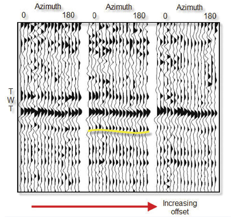
By stacking seismic data on the basis of azimuth it is possible to extract information regarding the relative magnitude of HTI anisotropy in the subsurface. By examining plots of traces sorted by common offset and common azimuth (COCA), event misalignment associated with HTI anisotropy may be evident (Figure 2).

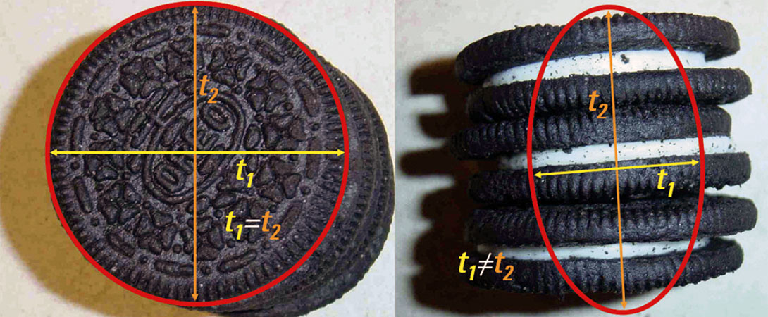
A common analogy used to illustrate the effects of HTI is based on Oreo cookies, where the delicious gooey cream filling represents fluids and/or rock gouge in fractures and the sweet dark biscuit represents the coherent rock between fractures. When Oreo cookies are stacked horizontally (Figure 3a) the seismic travel times through the stack in any direction are equal. If the cookies are aligned on their edges, however, the travel time paths form an ellipse where the shortest travel time is for paths that are aligned with the fractures as the energy can transfer entirely through coherent rock and avoid passing through the gas/fluid/rock gouge (Figure 3b).

The analysis of velocity variation with azimuth (VVAZ) and amplitude variation with azimuth (AVAZ) can provide important information regarding either fracture density and/or stress anisotropy. Both natural fractures and stress anisotropy are of critical importance to planning of hydraulic fracture stimulation, where much of the finding and development costs in shale gas plays are concentrated. Generally well log data is required to identify the source of the HTI as either aligned fractures, stress anisotropy or some combination thereof.

4. Reservoir Modelling and Geophysics: A Case Study from North-West Alberta

4.1. Geological Setting

The Triassic Montney Formation of the WCSB is a marine clastic rock deposited in a continental margin basin. The Formation comprises fine-grained (silt to shale) rocks with morphologically controlled interbedded sandstones. Carbonate content varies and can be locally abundant in similar proportions to quartz content. The Upper Montney comprises stacked sections of distal shoreface to shelf siltstones up to 150 m thick with laminae of pyrite bearing organic material (Hayes, 2009).

Due to the low (sub-millidarcy) permeability, horizontal completions and hydraulic fracturing are required to generate economic production levels. The economics of individual wells are generally improved by increasing the length of the lateral section and stimulating with multiple, separate hydraulic fracture stages. The very high costs of the stimulation are such that there is, justifiably, a strong focus on engineering in the development of the Montney Formation and other tight gas reservoirs. In this paper we present the case for utilizing geophysics, in conjunction with all other data, to understand lateral heterogeneity and optimize field development within the Upper Montney and Lower Doig Formations in an area of north-west Alberta between Grand Praire (AB) and Dawson (B.C.).

4.2. Petrophysical Data

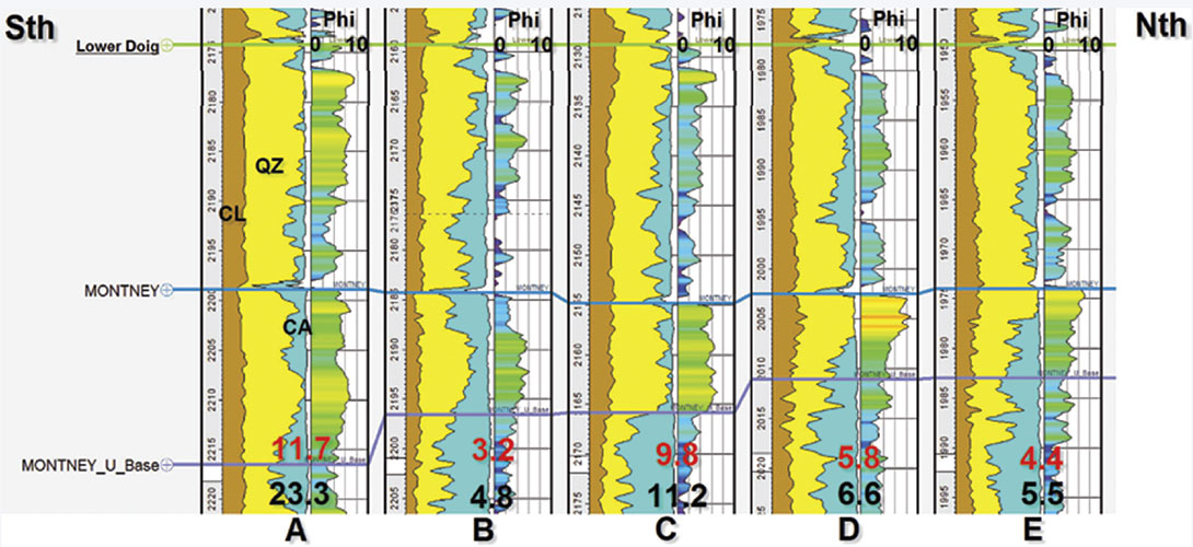
A total of 8 wells with density and sonic logs that penetrate the Lower Doig and Upper Montney formations were utilized in this study. Each of the wells was processed in a consistent manner (using the model described previously). The zone of interest in this area averages around 40 to 50 metres in thickness. Analysis of these wells through the zone of interest (Figure 4) illustrates the varying rock quality and thickness. The porosity-height values for the combined interval from the Lower Doig to the Base Upper Montney and for the Upper Montney only are included in Figure 4.

4.3. Seismic Inversion

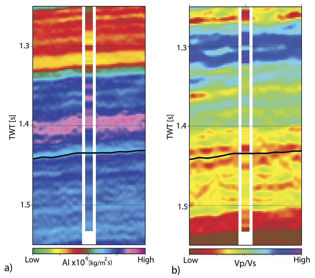
Using the ISIS simultaneous inversion algorithm four angle stacks (0-12°, 12-18°, 18-25°, and 25-30°) were inverted for acoustic impedance, Vp/Vs ratio, and density. The angle ranges for the four angle stacks were selected to optimize the fold, and hence signal-to-noise ratio, in each angle stack over the zone of interest. The extracted wavelet for the near angle stack and its associated synthetic is illustrated in Figure 5.

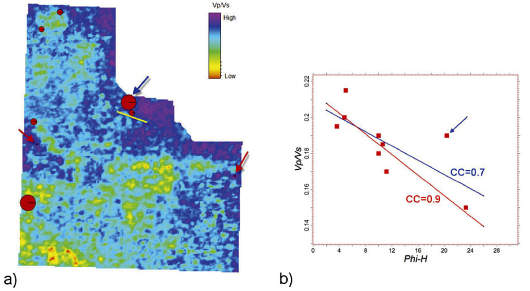
Results of the inversion for acoustic impedance and Vp/Vs ratio are illustrated in Figure 6, where they are compared to well log data from that location. These results exhibit a good correlation to well log data and confirm that the inversion is capable of predicting these properties. To test the hypotheses that the Vp/Vs ratio is a good indicator of reservoir quality, horizon or stratal slices through the Vp/Vs ratio volume are compared to porosity-height maps (Figure 7).

In general the Vp/Vs and/or Poisson’s ratio maps are a good indicator of porosity development within the Lower Doig/Upper Montney in the wells used in this study. However, in the absence of a larger dataset of wells this inference can not be backed up in a statistically meaningful manner. The AVO attribute map included in Figure 7 is only one of several possible and reasonable interval maps that could be created as hydraulic fracture stimulations grow in height to encompass tens of metres, and sometimes much more. Accordingly it is not unreasonable to include in our stratal slices a greater interval than that immediately surrounding our target horizon.

In addition to correlating inversion data to petrophysical estimates of porosity-height in this case study, micro-seismic monitoring results are also correlated with maps of inversion properties. Micro-seismic data are available in the study area from a horizontal well with an ~1100 metre lateral section in the north of the study area (Figure 7). The well was stimulated in five stages using a multi-stage open-hole completion, isolated with packers and ball-actuated ports. The treatments were monitored in a vertical well close to the centre and slightly to the north of the lateral section. The micro-seismic data recorded for stages 1 and 2 varies markedly from that recorded for stages 4 and 5 (Figure 8). No data were recorded for stage 3 as no fracture could be initiated, which is assumed to be a result of either a failure with the completion mechanism (although there was no conclusive evidence of this), or of changes in reservoir properties that increased the break-down pressure of the formation beyond that of the tubular limit imposed.

Figure 8 illustrates that relatively few micro-seismic events are recorded from stages 1 and 2 relative to stages 4 and 5, and additionally the distribution of the points is also markedly different. The concentration of micro-seismic events measured during pumping stages 1 and 2 to the north of the lateral suggest an asymmetric fracture propagation that created a complex, potentially less effectively-connected swarm of induced fractures from which to produce. The events from stage 2 also concentrate in the same area as stage 1, which indicates that new reservoir is not being stimulated during stage 2. In contrast, a greater number of events, which on average have a larger amplitude, were measured during stages 4 and 5. The alignment of events from stages 4 and 5 is also much closer to the expected orientation based on knowledge of regional stresses.

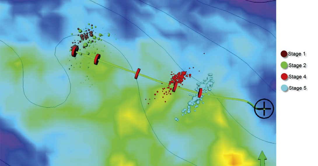
The stimulation stages were designed to be approximately equivalent in terms of total fluids and proppant pumped, the assumption being that induced fracture networks should be very similar for each stage. Although it is certainly possible that stimulation design and implementation practice, and not reservoir related properties, could explain the observations regarding the micro-seismic event patterns discussed above, we consider that changes in formation properties underpin the variable microseismic response. The increased Vp/Vs ratio indicated by the AVO results around the stage 3 frac port suggests that a higher breakdown pressure would be expected due to increased clay mineral content, and this may explain the failure to initiate a fracture for this stage. Stages 4 and 5 are located in a more extensive area of lower Vp/Vs ratio (Figure 8), typically representative of higher relative quartz content, which explains, at least in part, the improved stimulation results.

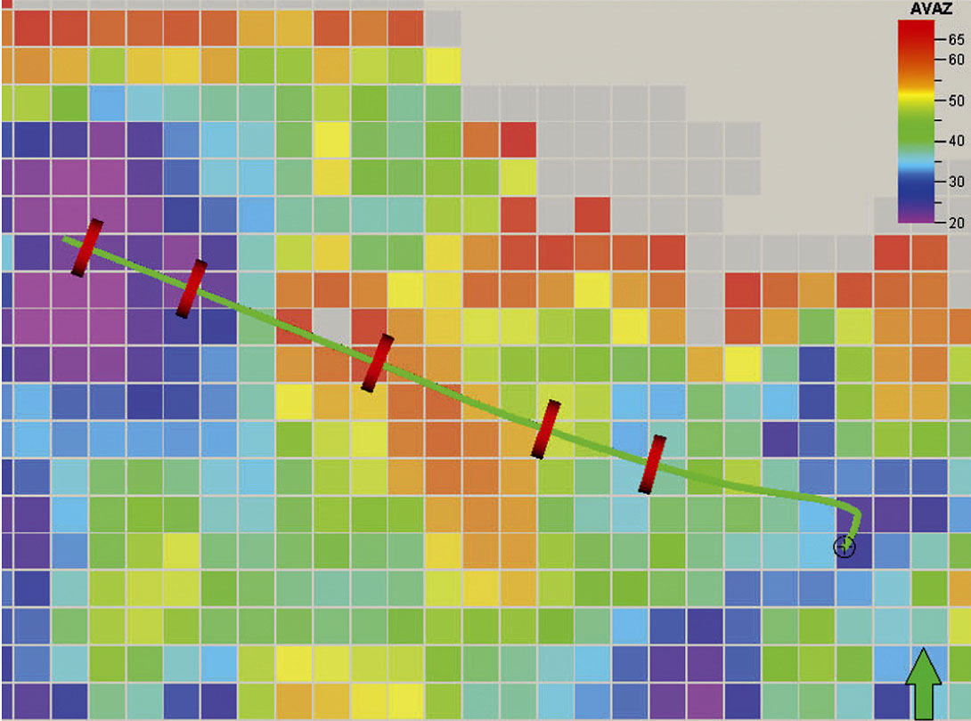
A possible alternative and/or complementary interpretation of the micro-seismic data pattern can be found in the amplitude versus azimuth (AVAZ) data. These data provide an indication of the degree of azimuthal anisotropy of seismic amplitudes. The anisotropy indicated by the AVAZ is substantially higher (by a factor of ~2) towards the heel of the well (i.e., stages 4 and 5) relative to the toe of the well (i.e., stages 1 and 2) (Figure 9). However, as the well is located near (<500 m) the northern limit of the survey the azimuthal distribution of data is imperfect and the consequence of this on the results is difficult to quantify. Regardless, we can say that for this example there is a strong empirical relationship between induced fracture complexity and AVAZ anisotropy.

4.4. Stimulation

Hydraulic fracture stimulation is critical to the economic production of tight gas and shale gas plays. Increasing the exposed surface area and volume of rock around the wellbore that is stimulated, and therefore capable of contributing to production, drives down the lifting costs of development. This makes stimulation efficacy a key focus of development. Horizontal drilling is a key and obvious means of contacting greater amounts of reservoir, and has been the single most critical step in the economic exploitation of tight gas and shale gas plays. In addition to horizontal drilling, advances in completion and stimulation technology have provided means of contacting greater volumes of reservoir. Optimal stimulation strategies can be formulated according to geological and geomechanical conditions. The choices of fluid type, additives, proppant size and concentration, pumping rates, monitoring and diversion technology are generally dictated by material and operational costs and how any modeled or perceived increase in production offset these costs over the economic life of the well.

The stimulation detailed in this case study utilized gelled “frac-oil”, a refined gas-condensate, which is perceived by some reservoir engineers to result in less damage to the formation as laboratory tests on core suggest the recovered permeability is greater for oilbased fluids. However, theory, and field results, indicates that the differential is short-lived and although the flow back of stimulation fluids may occur slightly more rapidly, the overall producibility of the reservoir is not improved by more expensive oil-based fluids relative to appropriately designed water-based fluids. Effective production is ultimately dictated by the conductivity contrast provided by the fracture, relative to the formation capacity to produce from the exposed surface area. The stimulation plan for this well called for each stage to pump ~50 tonnes of proppant; however, stages 4 and 5 ultimately received greater volumes, due to the available excess from failure to place proppant into the formation during stage 3.

The average volumes of proppant pumped in this area is currently between 80 and 100 tonnes per stage with associated bulk fluid volumes of ~200 m³. The current trend for wells exploiting the Montney Formation in western Alberta is to stimulate with foamed fluids, due to their capacity to hold proppant in suspension, efficiency in creating fracture volume (low leakoff rate), and relatively high retained fracture conductivity. Additionally, the bulk volume of fluid injected is either nitrogen (N₂) or carbon dioxide (CO₂), effectively limiting the volume of residual water to flow back. The increased viscosity of foamfluids relative to fluids such as friction-reduced water, or “slickwater”, results in better proppant transport and distribution within the fracture; whereas with slick-water as soon as fluid velocities are not sufficient to maintain turbulent flow that supports the proppant it drops to the base of the fracture. Fluid leak-off into the matrix adjacent the fracture-face is not considered an issue in shale gas plays, where permeabilities are in the nano-darcy range. Fluid leak-off can be an issue, however, in the Montney formation of western Alberta, as it is slightly coarser grained and in general has higher permeabilities (on the order of micro-darcies) relative to the more distal Montney Formation in eastern British Columbia.

Foam fluids are typically energized by N₂ or CO₂, and have surfactants added to increase viscosity. The gas fraction generally makes up approximately three-quarters of the total fluid volume and assists in increasing the viscosity (shaving foam makes an appropriate analogy). Due to the greater density of CO₂ relative to N₂, an equivalent volume of CO₂ foam delivers greater hydrostatic pressure, but the greater cost of CO₂ pumping may offset this advantage if the additional hydrostatic pressure is not required. Due to the greater viscosity of foam fluids relative to slickwater (Figure 10) an added advantage is that lower pump rates are required (~2 m³/min) relative to slickwater jobs (~8-20 m³/min). Foam fluid jobs therefore typically require less horsepower and machinery at surface, which partially offsets the greater cost of materials relative to slickwater treatments.

Where grain size decreases (and, therefore, typically permeability), and overall clay content increases in the Montney Formation in British Columbia stimulation strategies are generally more closely aligned with other North American shale-gas plays such as the Horn River Basin. In these plays, where nanodarcy permeabilities prevail, slick-water stimulations are the norm. This is partly driven by economics as slick-water is the lowest-cost stimulation fluid and the shale-gas plays require larger volumes of proppant so the discount of slick-water over gas is meaningful, but it is also partly a function of the formation response to stimulation. As the permeability of the rock in these plays is so low, there are very low leak-off rates, which leads to higher efficiency of fracture generation and the tendency to create complex high-surface-area fracture networks (at least in theory, real time micro-seismic monitoring or post stimulation logging are required to confirm such assumptions). The greater pump rates referred to above are required to maintain fluid velocity, and therefore proppant suspension as far as possible into the fracture network. Additionally, fine-mesh proppants are often substituted, sacrificing fracture conductivity to aid transport.

With the high costs of hydraulic stimulation raw materials (~$300/T for 20-40 sand proppant) and fluids, people and machinery (>$1M for a typical 6 -8 stage stimulation) the drive towards lean and efficient stimulation is inevitable, and will include increasing the length of laterals and the number of stages stimulated. This is primarily an engineering issue, however, if and where geology and geophysics can provide increases in efficiencies through improved understanding of the reservoir, the cost of this work will likely be paid out many times over.

5. Conclusions

Geophysics and specifically AVO inversion can bring significant uplift to tight gas and shale gas reservoir characterization studies. Variations in Vp/Vs ratio can be used to investigate and understand heterogeneity in reservoirs related to facies variations and changes in grain size and mineralogy. The AVO results presented here are correlated to both petrophysical modelling results from a number of wells and micro-seismic monitoring data from a single well. The continuation of this workflow is to integrate production data and decline curve analysis with volumetrics predicted from reservoir models based on log data at well locations and AVO inversion data between the wells.

Geophysical data, beyond simple horizon and fault picks, are needed to provide uplift and meaningful input in tight gas and shale gas plays. The potential benefits, in terms of mapping and well location high-grading, must be illustrated to asset teams reluctant to utilize geophysics. However, just as important as this is managing expectations associated with geophysical data and its interpretation by pointing out the limitations alongside the benefits and uplift. This case study delivers a single example of this, which provides a framework for the means in which geophysics can, and we believe, should be utilized in an integrated workflow.

*ISIS is a mark of Schlumberger

Acknowledgements

We would like to acknowledge the helpful and insightful comments and reviews by Richard Marcinew (Schlumberger Well Services) and the technical assistance of Maggie Malapad and Sean Johnston (Schlumberger Canada), and Greg Cameron (WesternGeco Canada). Richard Parker and Mike Jones (Schlumberger Canada) provided the micro-seismic data, via a cooperative anonymous client who we also thank. Patty Evans provided the seismic data from the WesternGeco Multiclient library and David Paddock (WesternGeco Houston) provided the basis of the Oreo cookie analogy.