Thomas Bayes versus the wedge model

Abstract

This paper demonstrates the use of the Bayesian inference to estimate model parameters in a synthetic example. The demonstration data are a set of zero-offset seismograms synthesized from a variation on the wedge model that thins in a general trend but with thickness that varies randomly about that trend. The velocity of the wedge layer also varies randomly about a mean with Gaussian variance. The presumed unknown is the bed thickness at each position along the wedge which we invert for using the maximum reflection amplitudes. Population of the amplitude/bedthickness joint probability density function, or likelihood, is achieved using Monte Carlo methods, while the Bayesian prior is provided by the presumed statistical trend and variance of the wedge thickness. The inversion result, or posterior, is a probability density function describing the wedge thicknesses probabilities. Results show that the maximum a posteriori parameter estimate is more accurate than the estimate found with the raw statistical trend or with a deterministic method of data inversion. Additionally, the posterior probabilistic density function can be used to perform statistical analysis, offering an avenue for quantified analysis of parameter uncertainty.

Introducing the contestants: Bayes

The Bayesian inference can be formulated as a mathematical theorem:

where P(A) is the probability density function (PDF) that describes the event A. P(B) is similarly defined. P(A|B) is the joint probability density function that describes event A given that event B has been realized. P(B|A) is analogously defined. The method of Bayes can be used to describe probabilistically the model space with the formalism

where m are the elements in model space and d are the elements of data space. Thus we seek the probability of a model given data. To do this we must know the probability of data given a model as well as the probabilities of both the models and data independently.

The PDF’s of Bayes’s theorem are named. P(m | d) is called the ‘posterior’ distribution, P(d | m) is the ‘likelihood’ function and P(m) is the ‘prior’ probability distribution. The denominator in equation (2) can be calculated as (Aster et al., 2005, p262:

where c normalizes the right hand side of (2) so that the integral of the PDF

over all models is unity.

A posterior PDF of possible models m can be found with measured data if the likelihood and prior functions can be established. Through a synthetic example we demonstrate a method of populating the likelihood function as a joint PDF (JPDF) between the model space and the data space. To do so the functional relationship between d and m must be known; which for us is the relationship between an Earth parameter and a seismic data response. Such a relationship might not be deterministically definable. For example, a rock physics model might relate porosity to the seismic amplitude at the top of a sandstone reservoir. However, since the amplitude will depend not only on the porosity, but also on fluid content, shale content, fluid pressure, etc., it is a multi-variate relationship. Any given porosity value might give a range of amplitude values. This covariance between seismic attribute data and Earth model parameter is captured by the likelihood JPDF P(d | m).

In addition to the likelihood function, the Bayesian inference includes a prior PDF that captures a priori knowledge about the model. If there is no independent knowledge about the model, the prior can be treated as “uninformative”, where all model parameters are equally likely. However, if prior probabilistic knowledge can be established, the resulting posterior can be designed to lend favor to results that are more probable given the prior knowledge. In our hypothetical example, such a priori information about the Earth parameters might come from a geological or statistical model.

Introducing the contestants: the Wedge

Our problem to be solved is that of estimating the thickness of a hypothetical thin bed wedge using convolutional zerooffset synthetic seismograms. The wedge is complicated by the fact that its thickness and the P-wave velocity have some random variation. To construct our wedge, the bed-thickness and velocity are assigned random values following the prescribed trend.

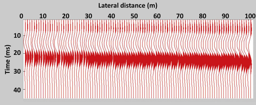
The model, which has a width of 100 m, is illustrated in Figure 1. The medium overlying and underlying the wedge has a constant density and velocity of 2400 kg/m³ and 3200 m/s, respectively. The wedge has an average trend of increasing mean thickness from 8.0 m thick on the left side to 18.0 m thick on the right side and has a normal random standard deviation around this trend of 2 m. The velocity also varies normally with a mean of 2500 m/s and standard deviation of 100 m/s. The density in the wedge is a constant 1700 kg/m3. The resultant density and sonic log at each position along the wedge are used to create a reflectivity series which is convolved with a 30 Hz Ricker wavelet to provide the synthetic data set illustrated in Figure 2.

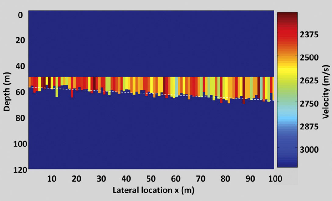
In this wedge, with a mean velocity of 2500 m/s, a 30 Hz signal has a wavelength of approximately 83 m. If, as noted by Widess (1973), a bed is tuned when its thickness is ¼ of a signal’s wavelength, our model bed thicknesses will be at or below tuning. Widess (1973) showed that below the seismic tuning thickness, the time-difference between the first seismic event and the second event may not indicate true bed thickness. However the reflection amplitudes can still be a bed thickness indicator and these amplitudes are used in our inversion.

In our problem, it is assumed that the following are known:

• The wavelet,
• The statistical trend and variance in the wedge thickness,
• The mean velocity and variance in the wedge.

This information can be incorporated into the Bayesian inference to probabilistically estimate bed thickness. The trend in the thickness of the wedge and the variance are representative of data that might come from geostatistical analysis. Likewise, the mean and variance in the velocity of the model could also be representative of statistical information derived from wells in a field data set.

Building The Likelihood Function

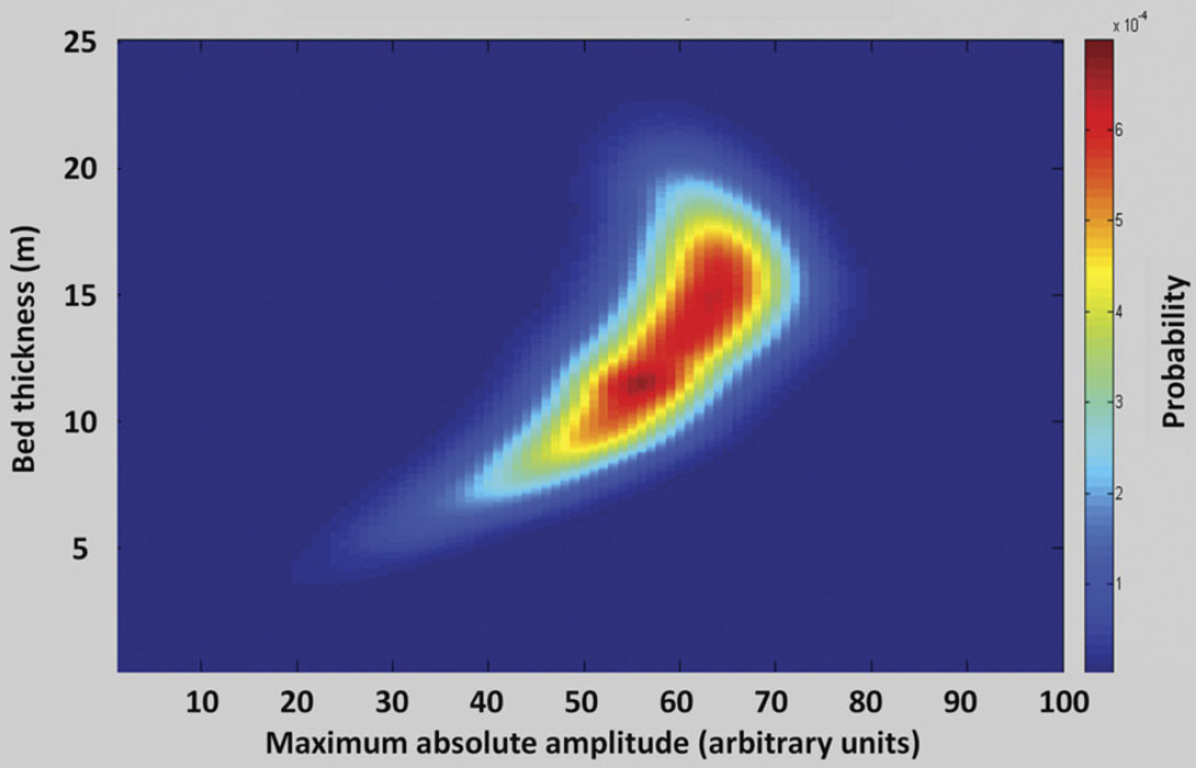
For our inversion, the “data” is the maximum absolute amplitude of each trace. The likelihood, P(d | m), is the multi-variate JPDF relating variables in model space (bed-thickness) and in data space (maximum absolute reflection amplitude). Our method of estimating this relationship is to sample randomly (i.e. Monte Carlo sampling) from the full multi-variate model space (bed thickness and bed velocity) and to calculate the corresponding point in data space. Repeated model space realizations and the corresponding data points build up the statistics needed to estimate the likelihood JPDF.

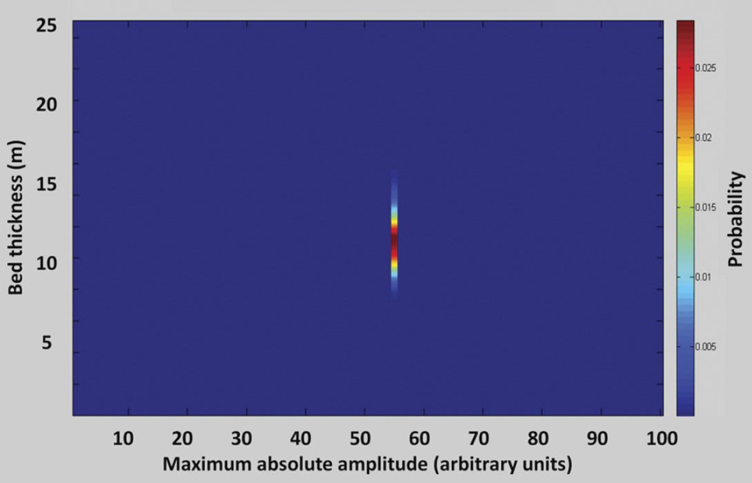
Specifically, we first construct a single thin-bed model with a bed thickness and bed velocity selected randomly using Monte Carlo sampling from the known statistics of the bed thickness and velocity. From this random realization, a synthetic seismogram is generated and a point in data space is populated with a corresponding point in model space (i.e. the bed thickness realization). The procedure is repeated a large number of times to provide the statistical population needed to estimate the likelihood JPDF. The likelihood JPDF thus generated is smoothed with a Gaussian smoother to eliminate bias introduced by discrete sampling from model space as described by Silverman (1986). Figure 3 illustrates the final likelihood JPDF generated from 5000 model realizations.

The Posterior with an uninformative Prior

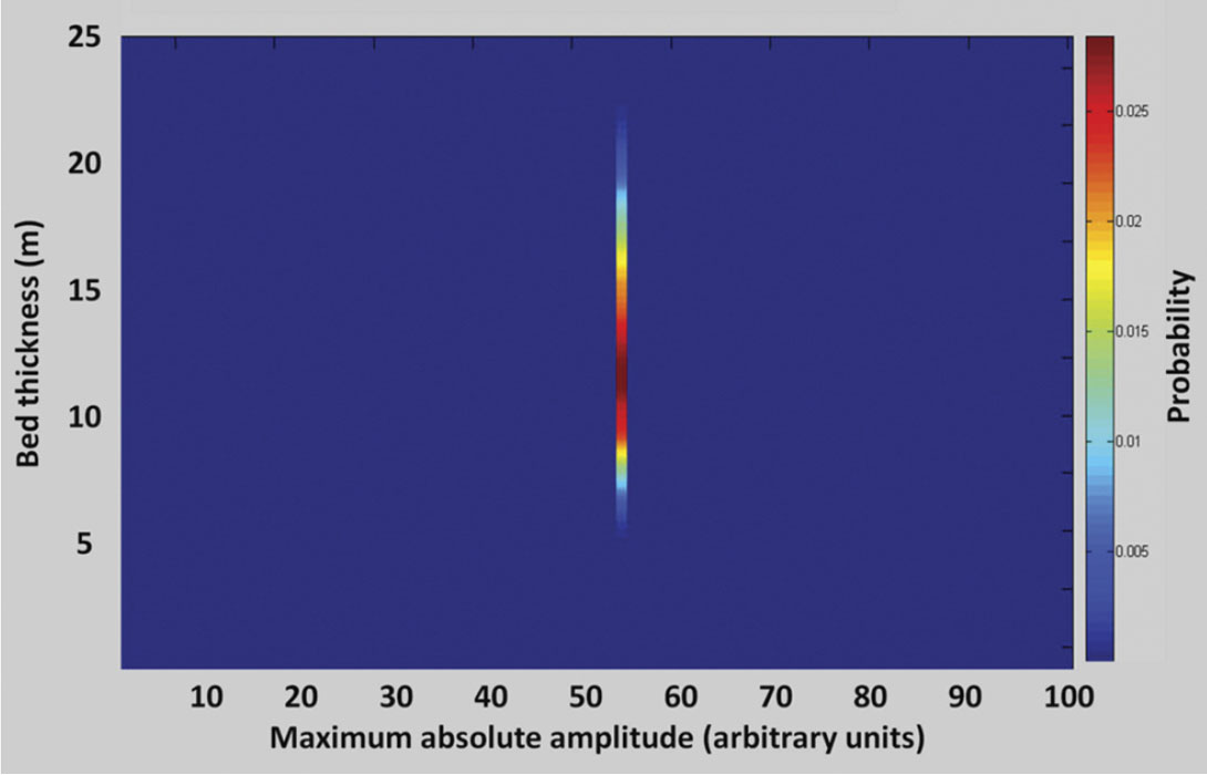
Having established the likelihood, we would like to evaluate the posterior. In Equation 2 the posterior is proportional to the product of the likelihood and the prior. If we assume that we have no prior knowledge about probability of possible models and we do not want to prejudice the model solution with information beyond that available from the measured data, then all models are assumed a priori to be equally probable. In this case, the prior is uninformative and set to unity. We can evaluate the PDF of model thickness at all locations along the wedge given the measured data by taking the PDF from the likelihood JPDF (Figure 3) that corresponds to the specific measured data. Figure 4 illustrates the calculated likelihood in the middle of the wedge. The denominator in equation (2) provides the normalization required to make the total cumulative probabilities equal to unity.

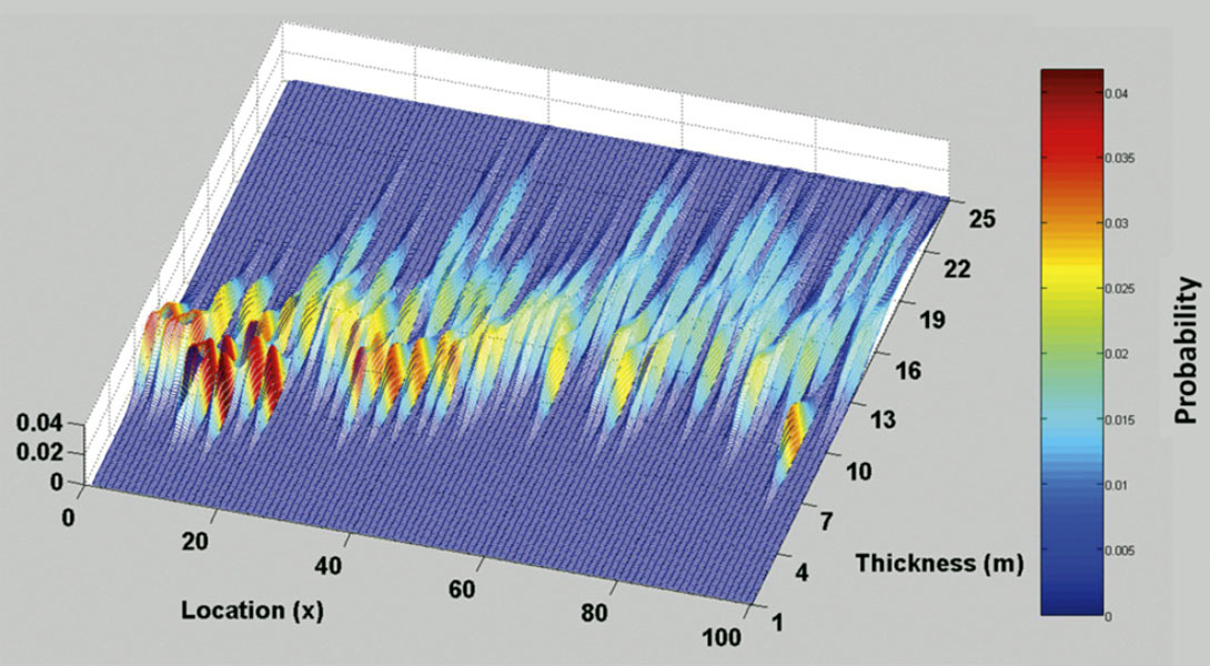
Similarly, utilizing the measured maximum absolute amplitude, the PDF of bed thickness can be evaluated at all trace positions along the wedge. Figure 5 illustrates the total solution across the model wedge. It is noteworthy that while each PDF has a bed thickness with a maximum probability, there is significant spread in the PDF’s because the data alone provide a poor constraint on the estimated bed thickness.

The Posterior with an Informative Prior

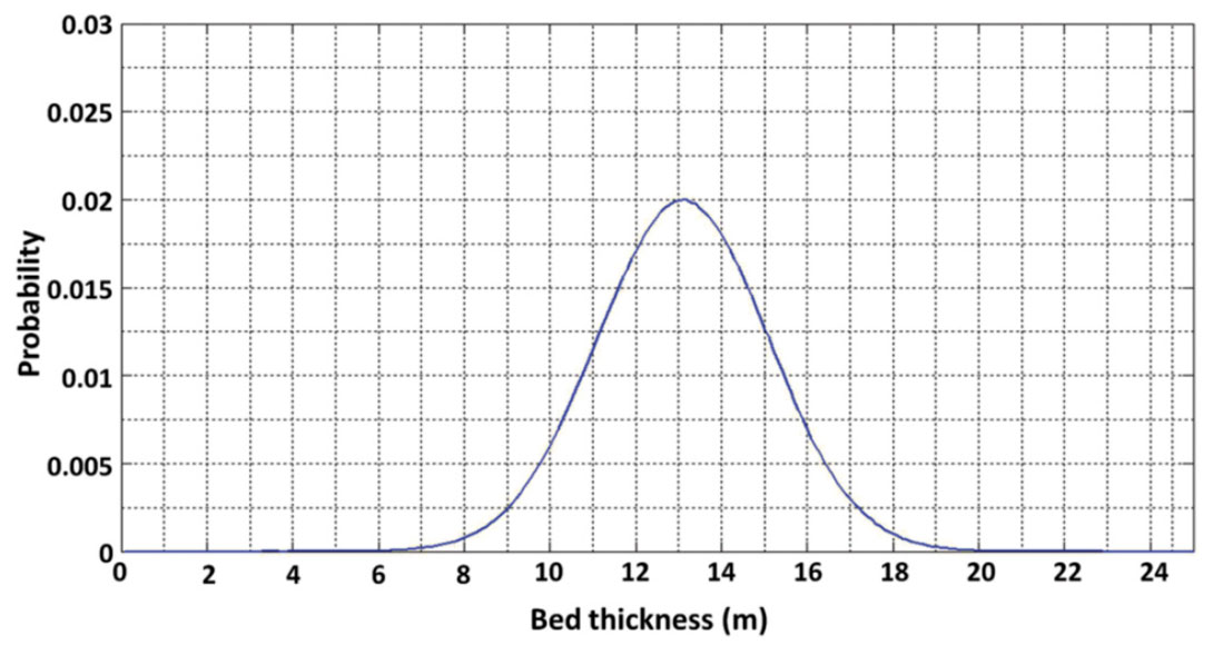
However, our knowledge about the wedge thickness is greater than that illustrated in Figure 5. We have prior knowledge about the trend in the wedge that we can include in the inversion via an informative prior. At each location along the wedge the prior P(m) can be defined by the known expected value of the bed thickness and the known standard deviation around this expected trend. For example, Figure 6 illustrates the prior in the middle of the wedge (x=50m) where the bed thickness has an expected value of 13 m and a standard deviation of 2 m.

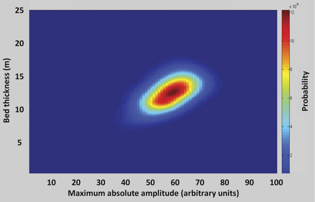
In Bayes’ theory the posterior is proportional to the product of the likelihood and the prior. To generate a posterior function with a weighted prior, the likelihood function from Figure 3 is multiplied by the prior function at each model location. An example of the posterior for the full model space in the middle of the model (x=50 m) is illustrated in Figure 7. Again, the specific PDF for bed thickness at this location is established by selecting the distribution corresponding to the specific maximum absolute amplitude from the data set, as shown in Figure 8. Figure 9 illustrates the PDF of bed thickness across the entire wedge, calculated with the informative prior which shows the bed thickness estimates to be much more constrained than the result illustrated in Figure 5.

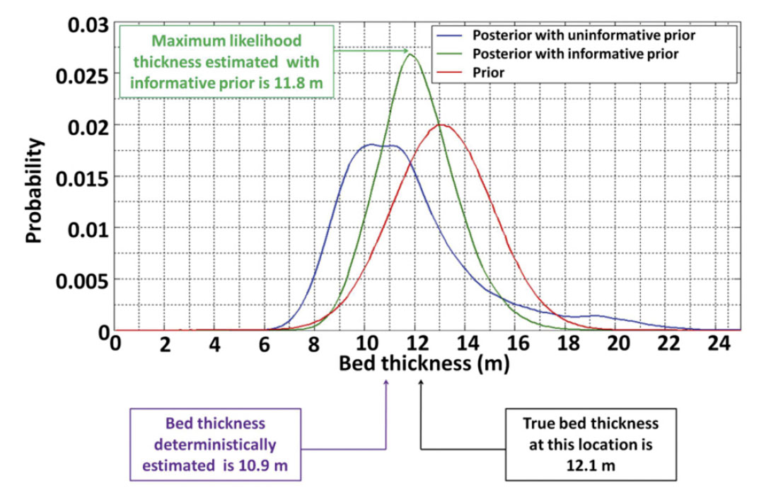
For a bed below the tuning thickness, Widess (1973) gives the maximum absolute amplitude of a composite reflection from the top/bottom of the bed as

where A_o is the amplitude of the reflection if there was a single reflector (i.e. a two layer model), z is the bed-thickness, f is the dominant frequency of the wavelet, and v is the velocity of the bed. Using Equation 4 the thickness of our tuned bed could be calculated from the absolute maximum amplitude of the seismic events if we assume we know the wavelet amplitude, the mean velocity and density of the wedge and further assume that the wavelet frequency is the peak frequency of the Ricker wavelet used to generate the seismograms. This direct inversion of the data would yield a deterministic estimate of bed thickness. Figure 10 illustrates how this deterministic estimate compares to the bed thickness estimated from the prior PDF alone, the posterior PDF with an uninformative prior, the posterior PDF with an informative prior, as well as the true bed thickness at the location in the middle of the wedge. The PDF’s can be used to estimate a maximum likelihood model result which is the bed thickness with the highest probability of occurrence. Figure 10 illustrates that the bed thickness with the largest probability from the posterior with the informative prior, called the maximum a posteriori (MAP), offers the best estimate of the true bed thickness.

Discussion

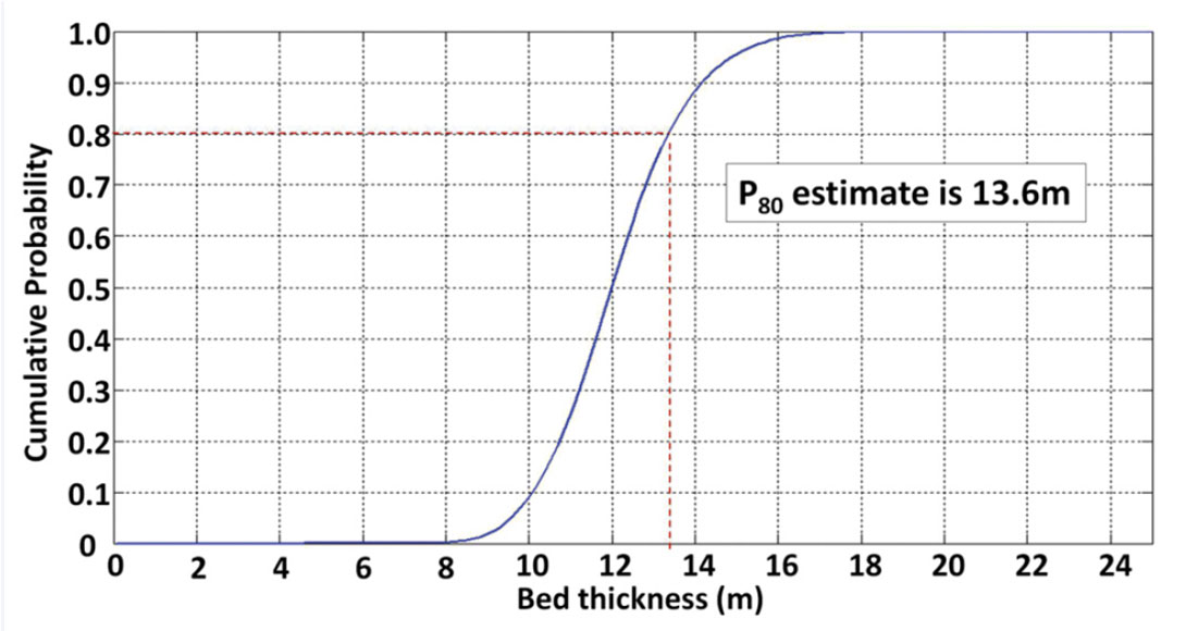
The posterior PDF for bed thickness has several utilities. Firstly, the maximum a posteriori can be used as the most probable single value estimate of bed thickness (Figure 10). Additionally, the posterior PDF enables quantification of probabilities within model space. For example, the cumulative probabilistic distribution of possible thickness values can be found. Figure 11 illustrates the 80th percentile bed thicknesses estimated from the posteriori PDF at the example location in the middle of the wedge (i.e. the wedge has 80% probability of being less than 13.6 m thick or 20% chance of being greater than 13.6 m thick).

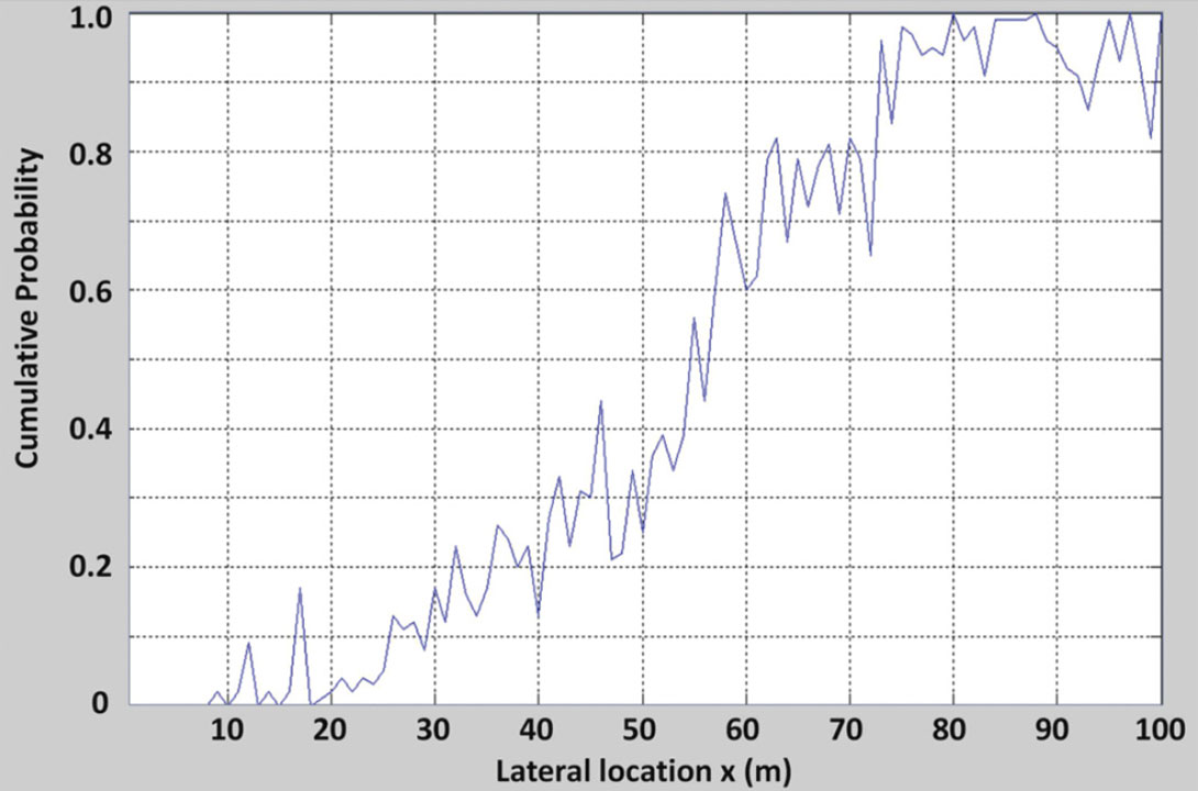
Also, the PDF can be used to establish the probability that the bed-thickness is at least as thick as a given value. An example of this form of analysis is illustrated in Figure 12 that shows the estimated probability that the bed-thickness is greater than a 13 m at each trace position across the wedge.

Other examples from Literature

Sava and Mavko (2007) derived a JPDF of fracture density and seismic data signature using a Monte Carlo simulation of the rock physics parameters. The JPDF related crack density to seismic amplitude variation with azimuth(AVAZ). The PDFs of the rock properties such as crack density, crack aspect ratio, fluid properties in the cracks were known and the JPDF of P-wave velocity, S-wave velocity, and density were derived from log data. Monte Carlo sampling was used to populate the JPDF between the crack density and AVAZ seismic response. The prior was established with the assumption that the probability of encountering fractured rock would decrease with increasing distance from a known fault. Multiplying the crack density/AVAZ JPDF with the prior that was established based on geological trends generated from the posterior JPDF. Additionally, their likelihood function was able to account for noise in the data.

When inverting for porosity, shale content, and water saturation in a reservoir, Spikes et al. (2007) constructed the likelihood PDF by comparing the seismic traces to an exhaustive set of synthetic traces generated from a complete but discretized set of rock property values. The subset of synthetic traces that had a sufficiently high cross correlation with the real traces was included in the PDF calculation. The result was a PDF for the possible geological models that could have yielded the measured trace.

Mukerji et al. (2001) used a Monte Carlo simulation to generate a PDF relationship between seismic facies and offset dependant amplitudes. The inversion result was a PDF of facies models.

Conclusions

The Bayesian inference provides a technique to integrate prior statistical information into a parameter estimate based on geophysical data. Statistical trends can be used to weight the prior in the inference and thus move the posterior PDF toward the a priori more likely solutions. This yields an improved maximum probability parameter estimate and the posterior PDF can be used to perform probabilistic analysis of model scenarios and possibilities.

Acknowledgements

This work constitutes a term paper submitted by Jason McCrank as a component of a graduate course on inverse theory taught by Dr. Gary Margrave at the University of Calgary. Jason’s graduate work, supervised by Dr. Don Lawton, received financial support the sponsors of the CREWES Research Project, Penn West Energy, SEG and CSEG.