The Winds of Change: Anisotropic Rocks – Their Preferred Direction of Fluid Flow and Their Associated Seismic Signatures

The Context of our Community

All of us interact in the context of our community. SEG and AAPG have played major positive roles in the community wherein I have worked for the last 30 years. These two societies invited me to speak upon a topic of my choice, for the benefit of our joint communities, and so this paper came into existence.

The “winds of change” refer to much more than just anisotropic rocks whose seismic anisotropy provide insight into permeability anisotropy. The way we view our planet is changing: the planet is now being studied as the interaction of interlocking systems. The four systems are: the hydrosphere, the atmosphere, the lithosphere, and the biosphere, as all of us absorb energy from our sun. The planet and all its subsystems, like geology or the weather, are explicitly evaluated as inter-dependent and interacting within the context of the local community. The heterogeneity at the surface of our planet and the re-cycling of compounds and elements (water, nitrogen, sulfur, carbon dioxide, etc.) enable our planet to support life. (See Our Changing Planet, McKenzie and McKenzie, and James Lovelock on Gaia for a farther point of view). Those of us in our 50’s have experienced two earthscience revolutions: the plate-tectonic revolution during the 1970s, and today’s profound re-evaluation of “how our planet works” and what our role as planet-dwellers is.

The rocks that are the primary focus of most of our studies are best understood as, firstly, the result of the interactions of the climate, the water conditions, the depositional setting, the biosphere, and the provenance of the sediments, and secondly, the lithification and geologic history they have undergone. The biosphere shows up in our rocks as fossils, one of our key means of dating rocks. We understand any given stratigraphic facies in the context of its spatial neighbors – its community — and its plate-tectonic setting. The climate includes the actions of gravity, sunlight, and atmosphere, but it is affected by where the land masses are, and how they are linked up together. The oil industry geoscientists are uniquely placed to have important data and tools to document the interaction of these four spheres throughout the last 660 million years and thereby track global climate change. The more-forward looking of our scientists and our oil companies are already doing just this.

Heterogeneous and Anisotropic Rocks: Do they veil or reveal the reservoirs we seek?

The sedimentary rocks wherein reside most of our supply of hydrocarbons are neither homogeneous nor isotropic, but instead are heterogeneous and anisotropic. Heterogeneous means spatially variable in property value: velocity, porosity, permeability, shale volume, sand percent, etc., and so the issues of spatial resolution and temporal resolution come to play. Anisotropic refers to the measured value being dependent upon the azimuth in which the direction is made. Reservoir detection and reservoir characterization encompass the mapping of both the heterogeneity and the anisotropy, in the context of the structure setting. Therefore, it is necessary to depict in map form at least 3 numbers for any property “of interest”:

1. the value itself (example: the large AVO gradient, the fast Interval Velocity, etc.)

2. the azimuth wherein the large value was measured.

3. the azimuthal difference in the value ( Vfast minus Vslow; Large AVO gradient minus Small AVO gradient; etc.)

Proper geophysics would also include the error bars associated with the measurement, or the goodness of fit of the field data to the ellipse that we consider field data “ought to show” in the presence of azimuthal anisotropy, so now we are up to four values per measurement of interest, all of which would be corendered into one icon (glyph or symbol that holds 4 numbers). Amplitude, interval velocity, coherence, frequency, phase, etc., are just a few of the geologically-significant seismic properties that have an azimuthal dependence.

The scale (frequency) at which the measurement is made determines the value measured, as well as the whether the rock looks homogeneous or heterogeneous or anisotropic or isotropic.

Anisotropy — like a Kitchen Sink

Anisotropy arises from the ordered heterogeneity(s) smaller than the wavelength. When the nature of the ordered heterogeneity replicates itself across different scale lengths (exhibiting fractal properties), then the anisotropy measured at one scale (the kilohertz frequencies – well logs) is similar to the anisotropy measured at another scale (the 10-100 hz reflection seismic). Just as a kitchen sink is a catch-all, so anisotropy as a term contains all the variety of the ordered heterogeneities smaller than the wavelength. What are the types or styles of order in the heterogeneities that we typically find in our rocks? Figure 1 shows the various ordered heterogeneities.

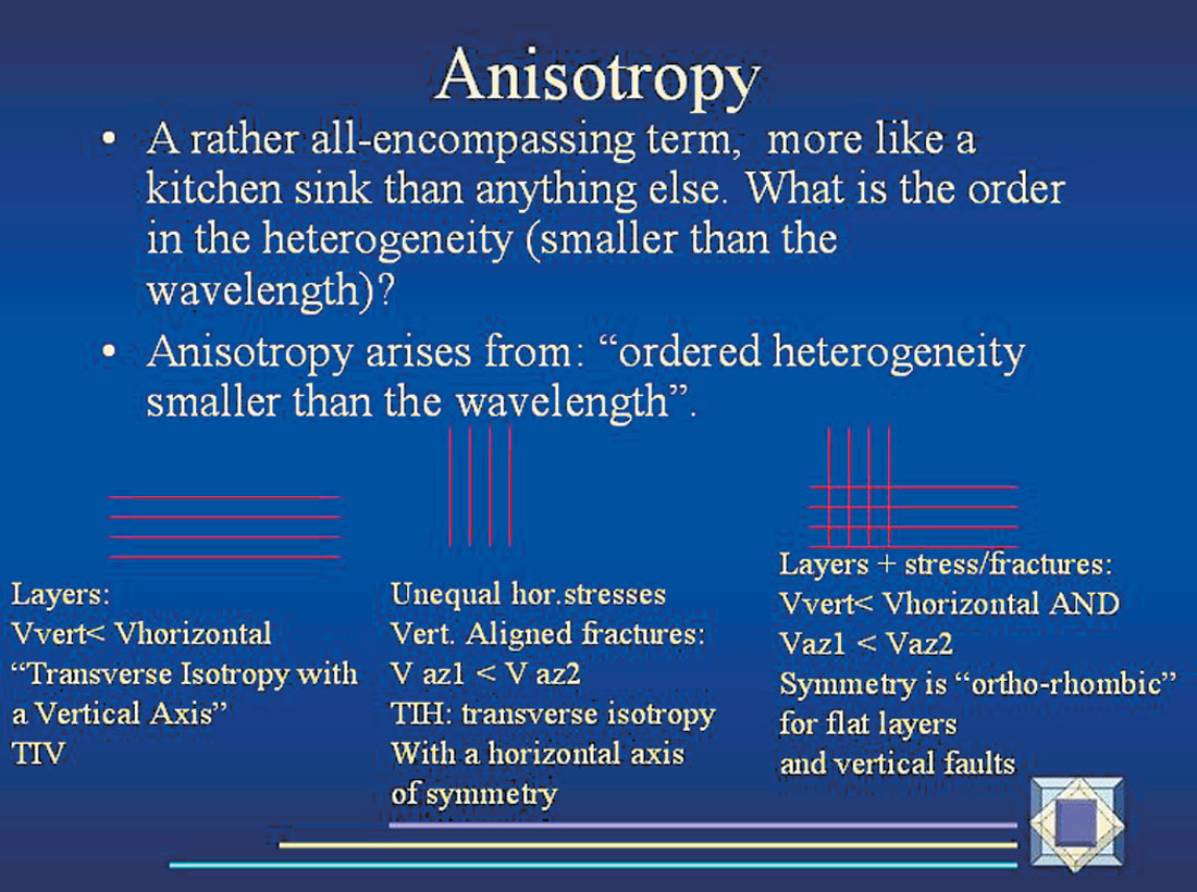
The layers of the sedimentary rocks exert the first order effect upon reflection seismic data. The vertical velocity is usually less than the horizontal velocity. This is termed transverse isotropy with a vertical axis, or TIV (or VTI). (This is like plates stacked in the sink.)

Vertical aligned fractures and/or unequal horizontal stresses cause azimuthal anisotropy. The P-wave velocity parallel the fractures is faster than the P-wave velocity perpendicular to the fractures. This is termed transverse isotropy with a horizontal axis , or TIH (or HTI). This symmetry is like the plates in the kitchen sink being stacked on end. TIH ignores the effect of the layers, which is not a good idea when dealing with reflection seismic field data.

The most reasonable symmetry model that the simplest of our rocks exhibit is flat layers plus unequal horizontal stresses and/or vertical aligned fractures, which results in orthorhombic symmetry. If there are two sets of vertical aligned fractures at 90 degrees to each other, this is orthorhombic symmetry too. The reason that some geophysicists are fixated on symmetry patterns is that the seismic waves acquire the symmetry of the rocks through which the waves pass. (Winterstein, 1990, 1992). So, if you want to know about the rocks, we need to know about symmetries. Don Winterstein (1990) wrote an excellent paper in Geophysics on this. One good fact about orthorhombic symmetry is that after identification of the fast direction and the slow direction, and azimuth-sectoring into these directions, then most “isotropic” seismic processing code can function fairly well on azimuth-sectored data. This is one reason why some people azimuth-sector: they don’t have to re-write their codes to use all the data all at once.

Many areas we explore in have dipping layers and/or dipping faults (dipping fractures). Therefore, monoclinic or triclinic symmetries would be expected. One consequence of monoclinic or triclinic symmetry is the misalignment of the azimuth of the fast P wave velocity and the fast shear wave polarization. Other consequences are less well understood, and more papers explaining to all of us what monoclinic and triclinic symmetries look like in field data would help.

Bill Abriel: Spring SEG DL 2004 – Complex Earth, Complex Tools, and Communication

Bill Abriel delivered a wonderful lecture on reservoir characterization that is the springboard for this work. Bill’s DL was webcast, which is how Walt and I heard it. Webcasting DL talks and all major society interchanges is our future, here now. Bill emphasized several fundamentally important points: we have a complex earth, we have complex tools, and we must communicate. Our complex earth has impelled us to develop complex tools. These complex tools rarely deliver visually clear interpretable results: we must interpret the results that our tools give us. We must show clearly what we do know and what we do not know, including uncertainties and ambiguities. To present what the seismic data tells us, we must capture both the heterogeneity and the anisotropy. This means, the spatial distribution of the measurement itself (velocity, amplitude, porosity, etc.) and its azimuthal variation, and the spatial relationships amongst all these measurements. Co-rendering of very high dimensional datasets is a key issue for our industry and will assume greater and greater importance, as more and more people deal with multi-azimuth multi-component 3D data.

The purpose of the communication of what we know and what we don’t know is to obtain consensus and co-operation, for the days of the Lone Ranger are gone. The asset teams bring together the joint disciplines needed to understand the reservoir.

Our Complex Earth

Our complex earth contains a continuum of all scales of ordered heterogeneities, from which arise the three types of seismic responses:

1. reflections : arising from layers – ordered heterogeneity – 3/8ths wavelength thick or thicker. Widess (early 1970s) wrote “How thin is a thin layer?” and the answer is: 3/8ths wavelength thick gives us a discrete reflection from the bed top and another discrete reflection from the bed’s base. These are the coherently reflected waves that comprise the classical “Signal” for processors.
2. Scattering (coda, trailing legs) and attenuation and dispersion (velocity is a function of frequency). When the ordered heterogeneities have scale lengths about 0.3 to 0.01 the size of the wavelength, then the seismic wave rattles around inside the fractured zone, with multiply scattered travelpaths. These are the “coda” or trailing legs that classical processors remove as Noise, using various forms of deconvolution.
3. Azimuthal variation in the traveltimes: effective media theory describes the change of velocity with azimuth and offset as though there were vertical aligned “penny shaped cracks” present, whose dimensions are much smaller than the wavelength.

Figure 2 presents the three seismic responses (reflection, anisotropy, and scattering/dispersion/attenuation) as a function of frequency and discontinuity size on a log-log plot. Frequencies from 10 hz to kilohertz (sonic) to megahertz (laboratory) measurements are shown. Discontinuity thickness (or size) ranges from microns to mm to meters to kilometers. The principal focus of my work here is in the 10-100 hz realm, although it is important to fit into a Unified Theory all the other seismic measurements (crosswell, passive seismic monitoring, sonics, and laboratory). A given set of vertical aligned fractures will cause anisotropy within one (low) frequency measurement, dispersion/ scattering/attenuation to a (mid-) frequency, and reflections to the highest frequency seismic waves. The seismic response one measures is the result of the scale of the ordered heterogeneities relative to the wavelength used.

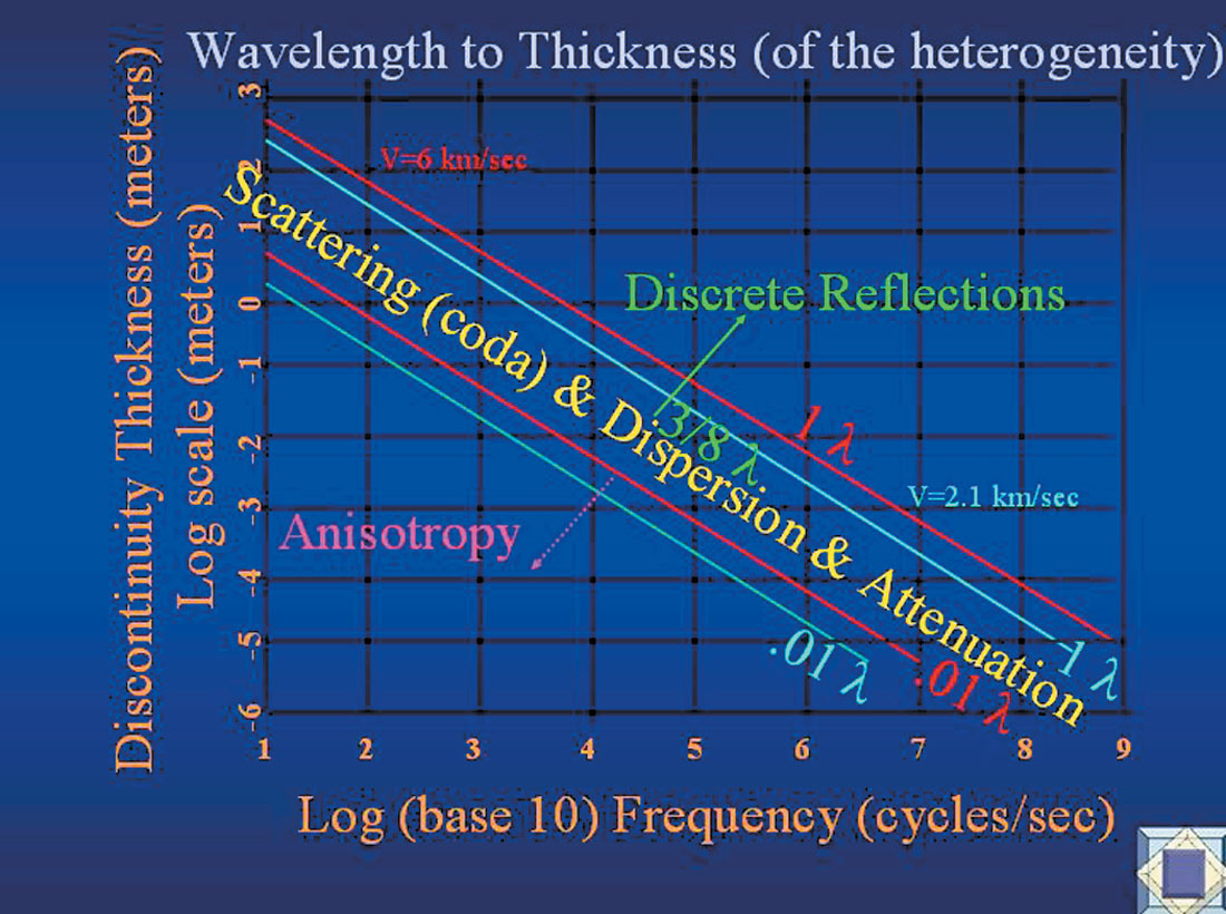
Figure 3 presents the well-known graph showing that velocity changes as a function of frequency. The conventional wisdom of our community understands this type of observation to indicate that the high frequency, higher velocity region is the unrelaxed state of the rock, where the fluids in the pore space can not equalize their pressure (move) as the seismic wave passes through: the seismic wavelength is much too short to effectively move the fluid around, so the fluid acts as a stiffening agent. The low frequency, low velocity region is the relaxed state of the rock, wherein the fluids can move between the pore spaces as the long wavelengths pass through, equalizing the pressures, and thus a slower velocity results. The transition zone between the two states is the zone of Dispersion (for velocity changes with frequency), attenuation, and scattering (coda).

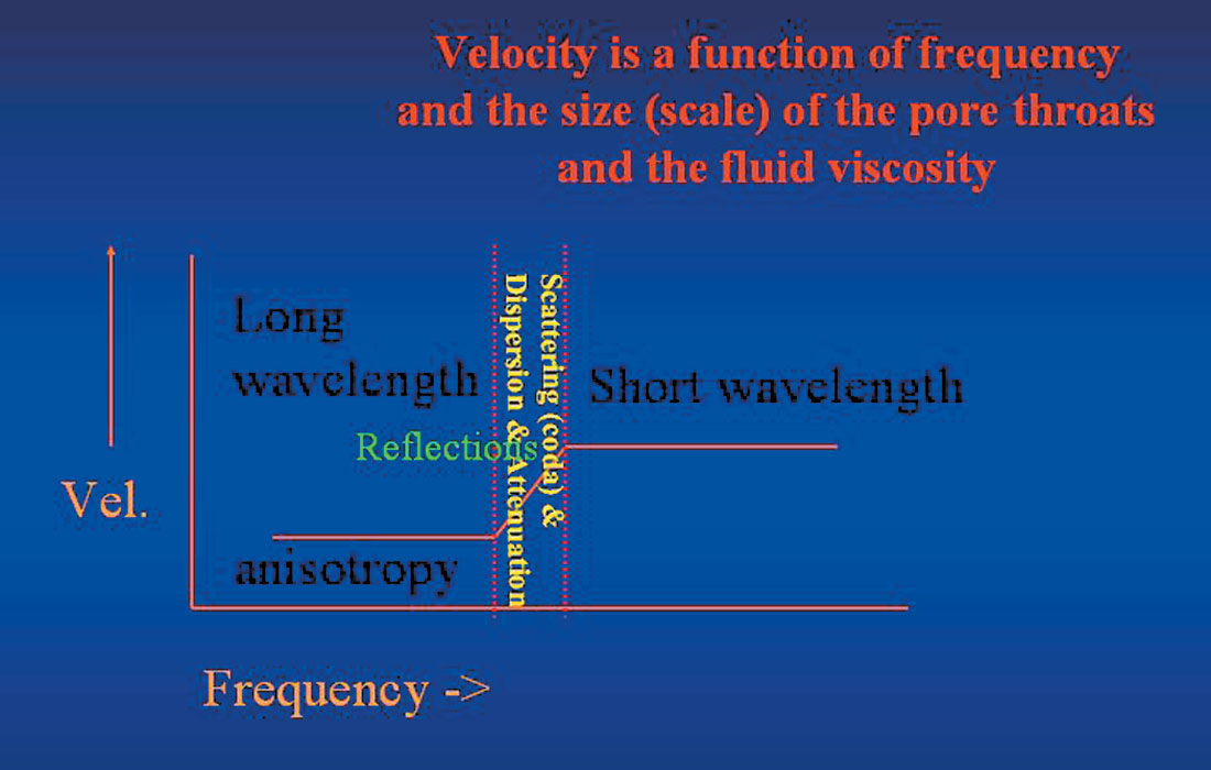
Therefore, it is possible to think about velocity being a function of frequency, as well as the scale (size) of the pore throats and the fluid viscosity, for the pore throat size and the fluid viscosity affect the flow rates through the rock. In the presence of high fracture density such that horizontal permeability anisotropy exists (preferred direction of fluid flow), then seismic anisotropy is present, as well as the potential to measure the dispersion, using surface seismic reflection data. The high fracture density, with fractures of scale lengths approaching the wavelength have introduced pore throat sizes much much larger than those present in unfractured rocks. With or without this effect, may be the azimuthal scattering effect, wherein parallel the fractures whose scale lengths approach the wavelength there is less scattering, and perpendicular these fractures there is more scattering, attenuation, and dispersion. The next Great Challenge in seismic anisotropy is capturing, displaying, interpreting, and modeling these field data observations.

Reflections (from thick layers)

Every 3D-PP migrated volume displays focused imaged reflectors. Interpreted reflectors give us maps of horizon dip magnitude and dip azimuth, using various measurements of coherence. Lineations on these maps are commonly observed and related to macro-fracture lineaments. Prof. Kurt Marfurt at the Univ. of Houston and his colleagues have developed a way to calculate 3D volume curvature from 3D migrated PP seismic data. Their displays of curvature can highlight subtle lineations in the 3D data, and can provide additional information pertaining to the study of fractures and fluid flow in reservoirs.

Reflections+Anisotropy (azimuthal variation in PP traveltimes)

Figure 4 displays the well-known azimuthal variation in traveltimes of the far offsets (offsets about equal to target depths). The azimuths displayed are from 0 to 360, which is the correct way to view azimuthal variations in seismic signatures. The all-azimuth ellipsefitting that uses all the data to determine the anisotropy is a powerful approach that captures the azimuthal variation in traveltimes and amplitudes. Sometimes people view the PP azimuthal traveltimes from 0 to 180, but too much information is lost that way. The variation of minimum time (fast) to maximum time (slow) over a 90 degree azimuthal variation is the classical signature of the “penny-shaped cracks” in the rocks above the reflectors that exhibit these azimuthal variations in traveltimes. The slide exhibits a “large” anomaly.

Not all Pores are Connected… Not all Fractures flow Fluids

We can find porosity (usually by inversion of amplitude into impedance). But how big are the pore throats? Pore throat size and fluid viscosity are involved with the effective permeability. The flow through a given length depends upon the cross section area (for flow), the pressure gradient, the fluid viscosity, and the permeability. A fractured reservoir with a horizontal permeability anisotropy has pore throats much larger than those normally encountered in conventional reservoirs.

We can find the relative density and orientation of “penny-shaped cracks” by mapping the azimuthal variation in PP traveltimes, or AVOaz, but do these fractured areas flow fluids?

There is additional information in our 3D wide-azimuth data, hereto- fore under-utilized, which should be captured and mapped, not removed in processing.

The Seismic Model Signature of Changing Permeability, from the Edinburgh Anisotropy Project

Chapman, Maultzsch, Liu, and Li, presented their work on frequency dependent anisotropy at the SEG/EAGE Summer Research Workshop, 2004, in Vancouver. They have been kind enough to let me show some of their slides. In Figure 5, we see their numeric model: a sandstone with VP=4090 m/s, VS=2410 m/s, density =2.37 gm/cc, with a fracture layer embedded inside it.

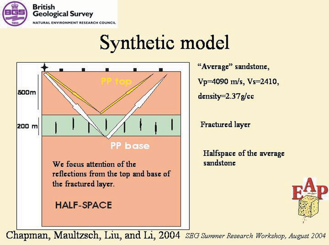
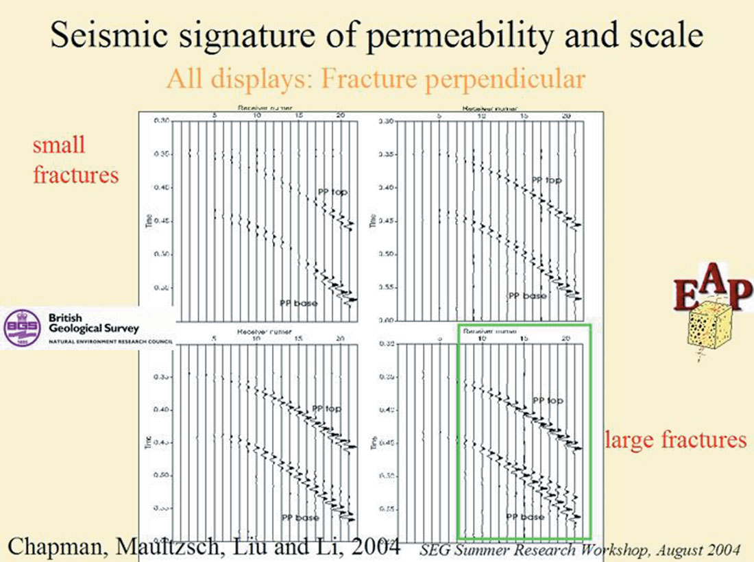
Figure 6 presents four different effective permeabilities, modeling from small fractures to large fractures (upper left to lower right). All four datasets are the fracture perpendicular direction, for the fracture parallel direction has minimal effect from the fractures. Only the mid- to far- offsets perpendicular to the fractures exhibit the effect of the fractures. As the fractures become larger, the effective permeability is greater, and the base of the fractured layer exhibits the dispersed signature that theory predicts. When the fractures are small, and not that permeable, then not much seismic effect is seen. The green box indicates the upper end of the modeled anomaly: the high frequencies have a faster velocity (less moveout), while the lower frequencies have a slower velocity ( more moveout). The green box indicates the region to be enlarged and displayed in Figure 7.

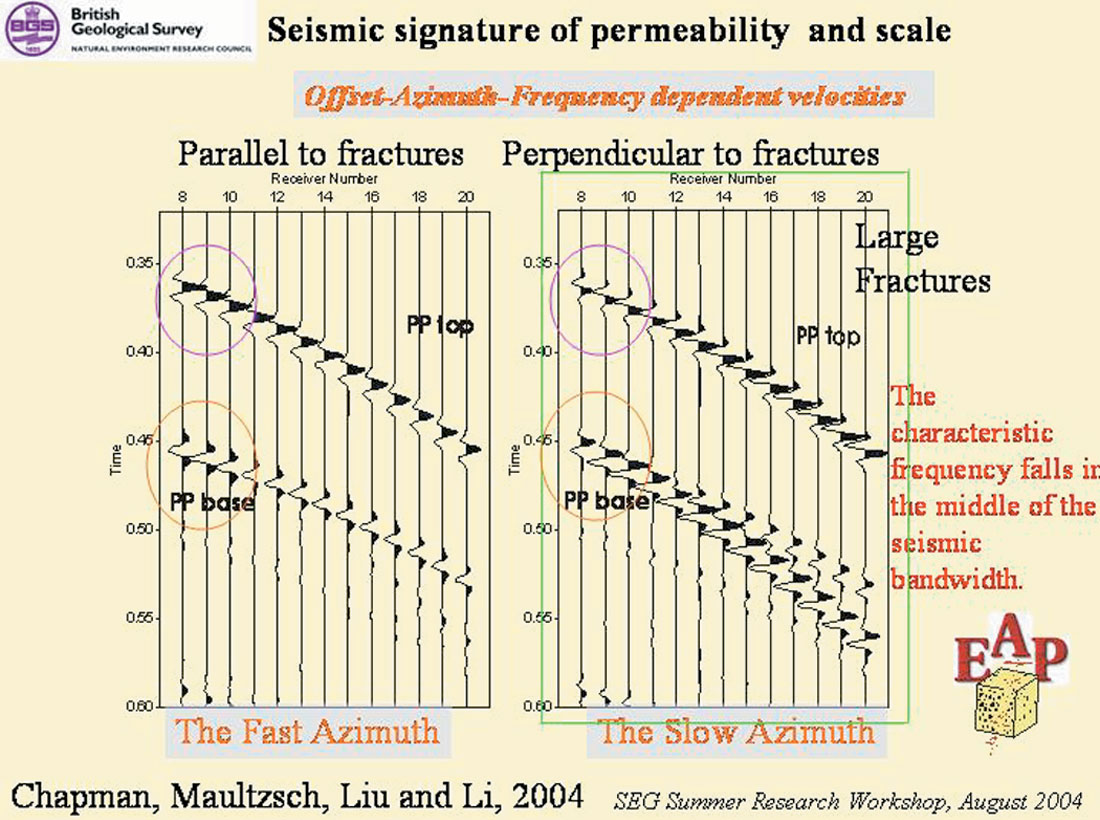
Now we can compare the fracture parallel and the fracture perpendicular signature, for mid-to-far-offsets. Figure 7 displays on the left the fast azimuth, parallel to fractures, with its zero phase reflection from the top of fractured layer at the mid-offset. On the right, is the slow azimuth across the fractures, with its 90 degree phase wavelet at the top of the fractured layer, at a mid-offset. The Base of the fractured layer again is zero phase in the fast direction, while at the mid offsets, it is more like a 90-degree phase wavelet. At the far offsets, the low frequency and the high frequency reflections are distinctly different, showing different moveout curves.

Obviously, what one would do to test for this phenomenon in field data is to acquire full azimuth full-offset PP 3D data, then separate by azimuths – fast and slow – and then band pass filter the SLOW direction into the low-half of the spectrum to run its own velocity scans. Then run a separate bandpass filter for the high-end of the spectrum, two octaves on each filter, please, and run its own velocity scan. While some might protest, “But this looks like a multiple!”, I reply that this is model data and has no multiples. I believe that people are clever enough to figure out how to get rid of the multiples and preserve the dispersion. (How’s that for optimism?) A good first step is to forget about trace-by-trace spiking deconvolutions, and to forget about spectral whitening, if you want to see the plumbing in your reservoir.

Of course, we have to get rid of the peg-leg multiples, the long-period reverberations that obscure our signal, but we just need to be careful how we get rid of them. Perhaps a surface-consistent gap deconvolution to remove reverberations could be considered, to leave the wavelet’s phase alone. The opinions about deconvolution are equal to the number of geophysicists in the room.

The importance of the difference in phase between these two different-azimuth sections can not be over-emphasized . The necessity to compare phase by azimuth in our field data can not be overemphasized. The non-unique interpretation step of azimuthal phase shall be discussed later in this paper.

Field Data: US Dept of Energy Wind River Project

Figure 8 displays some PP supergathers (3 gathers displayed as a partial-stack) in the East-West fracture parallel direction and in the North-South fracture perpendicular direction. The data come from the US Dept. of Energy Wind River project (naturally fractured gas reservoirs’ study). The CDPs of these gathers are the same ground locations. Please note the high frequency nature of the fracture parallel, while the fracture perpendicular shows more energy in a lower frequency range. Moreover, the low-frequency reflections perpendicular to the fractures clearly exhibits a slower NMO on CDP 83 at 1.55-1.60 sec, while the higher frequency reflections are clearly flat, due to proper NMO.

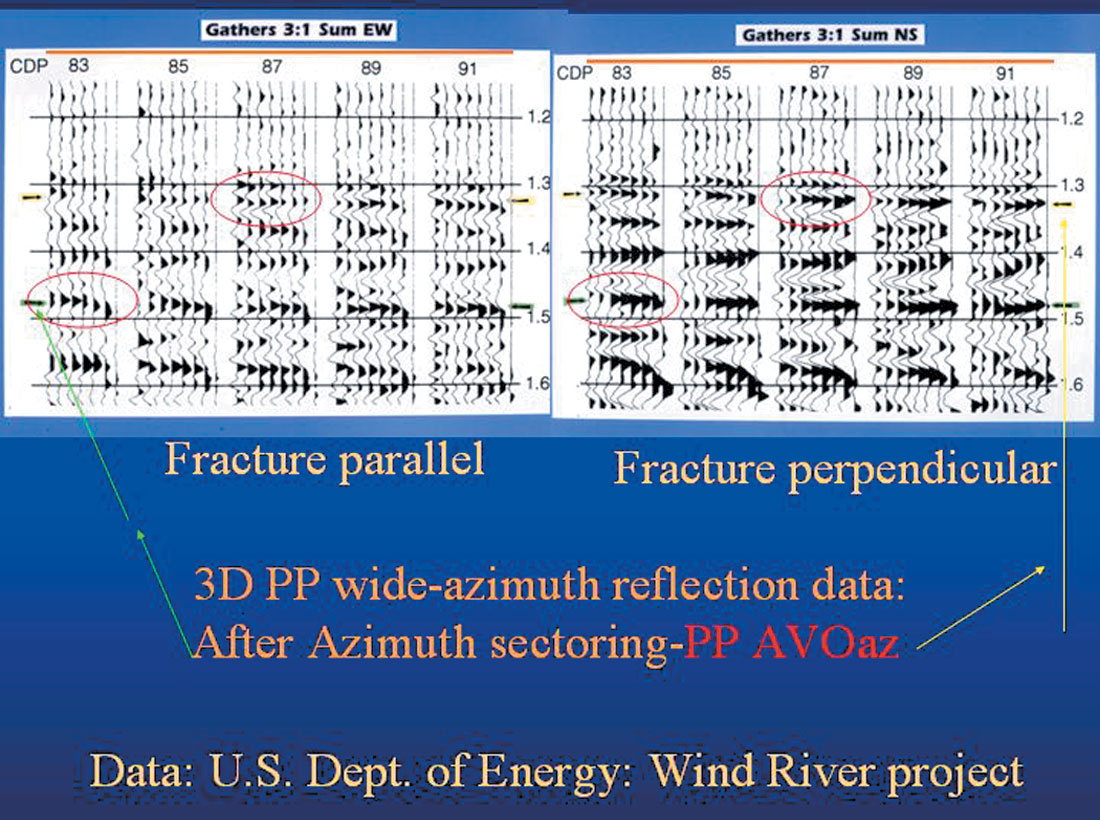
The arrows point to AVOaz anomalies studied in the earlier studies (Grimm et al., 1999; Lynn et al., 1996, 1997, 1998, etc.) At the time, we were not thinking about dispersion, but we should have been. Other geophysicists who viewed these slides, were: Dr. John Queen, who has been studying seismic anisotropy for over 20 years, asked perceptive questions when these slides were first shown. The low frequencies perpendicular to the fractures are indicating different moveout (slower) at 1.55 sec, while the higher frequencies are flat. This area also had different NMO velocities applied: E/W was faster and N/S was slower, just to get the gathers to appear as “flat” as they are.

Figure 9 shows the stacked migrated data for these gathers. In general, the E-W fracture parallel is higher frequency and lower amplitude; while the N-S fracture perpendicular is higher amplitude and lower frequency. Also please note the difference in apparent time structure for the CDPs presented here. The same ground locations (CMP bins) are presented, but the azimuths of their raypaths are different. Different velocity fields were used for moveout and migration, based upon the NMO curvature observed.

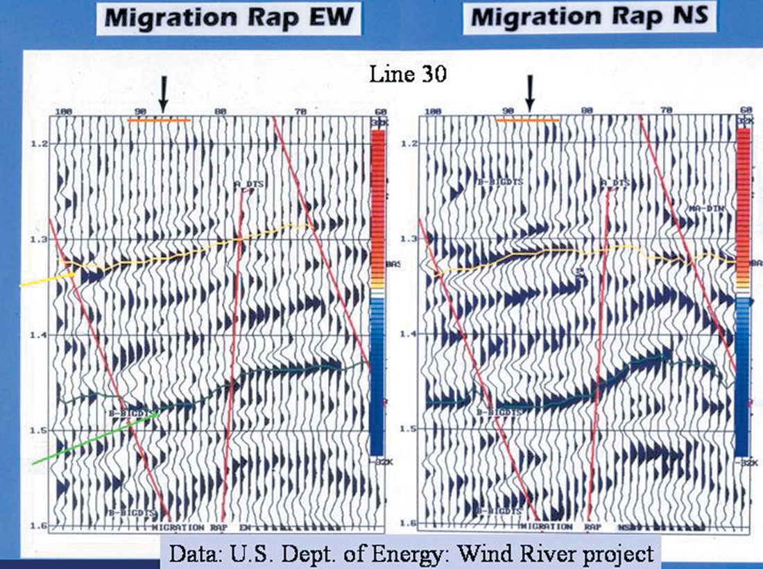
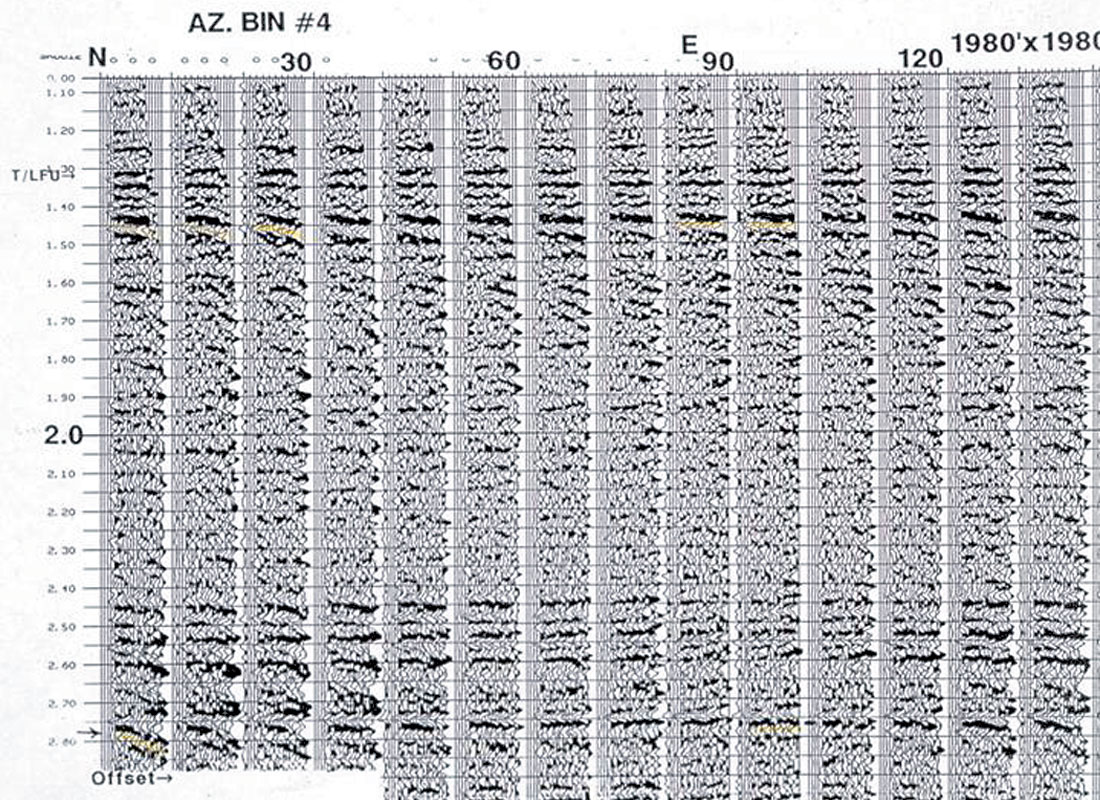
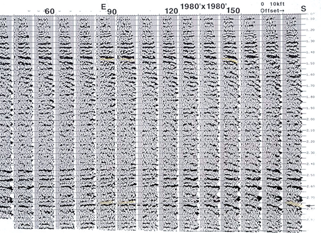
Figure 10 is from another area in the survey, and shows a supergather 1980 ft x 1980 ft. The azimuths range from 0 to 140 degrees, with each azimuth sector being 10 degrees wide. Only one PP NMO function was applied to all these data (and the rest of the data on Figure 11). Please note the flat high frequency E/W gathers at 2.4-2.7 sec, and have the minimum traveltimes on the far offsets, which indicate the fast, fracture –parallel direction. The N/S gathers have some high frequency energy that is flat, but much more low frequency energy that is slower and still needs more moveout. Figure 11 displays from 30 degrees to 180 degrees.

Other supergathers in this area showed dispersion in the PP reflection signatures on the order of 50 msec difference in traveltime at 4 seconds between the high frequency events and the low frequency events. (Lynn and Beckham, 1998).

These data were acquired in a naturally fractured gas reservoir, and it is probable that the cause of the dispersion is scattering off aligned vertical fractures whose scale lengths approach that of the wavelength. The fracture parallel direction is less scattered, while the fracture perpendicular direction is more scattered.

Where to Hunt

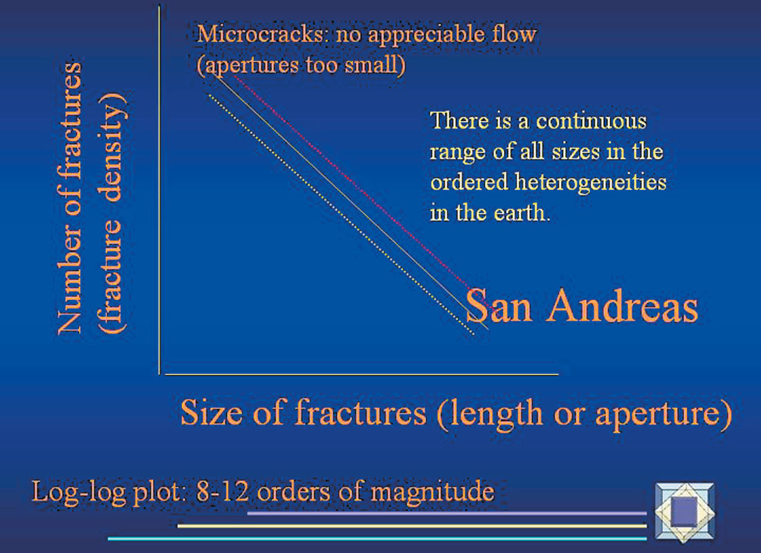
We don’t have to hunt Everywhere for offset- azimuth- frequency velocity (dispersion) effects. We only have to start the hunt where there is a good PP-AVOaz anomaly. Why? Many publications have documented the log-log relationship of number of fractures to size (length or aperture) of fractures, from the scale of the micro- fractures to the scale of the San Andreas. Figure 12 illustrates the continuous range of all sizes in the ordered heterogeneities in the earth. The “context of the community” is revealed upon this slide: our friends the geologists have documented the various scaling properties of fracture populations and we would do well to heed their insights.

I’m collecting published references to generic figures in this paper, to include in the References. Please email me your favorite papers that pertain to the generic figures in this paper.

An upper and lower bound of the scaling relationship between size of fractures (length, aperture) and number of fractures (per unit volume, usually). The lower bound is a “relatively” unfractured rock mass, while the upper bound is the “fracture criticality” fracture density that Stuart Crampin has defined. Fracture criticality is the threshold fracture density which, when achieved, results in an interconnected network of fractures, and a significant permeability uplift. Fracture density less than fracture criticality implies a fracture network connected only to the matrix porosity, and not to all the other fractures in the rock volume.

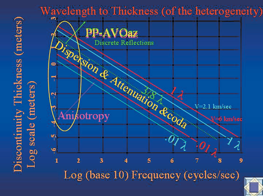
The magnitudes of the PP AVOaz anomaly are often 50-100% azimuthal variation on the far offset. This magnitude far exceeds the equivalent media theory (Ruger-Tsvankin, The Leading Edge, Oct. 1997) equations’ predicted magnitudes. Therefore, it is appropriate to ask searching questions about “WHERE?” are these large magnitude AVOaz anomalies arising from. Since equivalent media theory can not explain the magnitudes of most AVOaz anomalies, new/ better/ broader theories are needed. I suggest that “the context of the local community”, as demonstrated on Figure 12, 2, and 3, is a large part of the answer. Figure 13 displays the yellow oval of the PP-AVOaz response in the 10-100 hz bandwidth (our reflection seismic and VSP signals). It squarely overlays the zone of discrete reflections and anisotropy: already well-known as governing the nature of PP AVOaz responses. Right in the middle between the discrete reflection and the equivalent media theory regimes is the dispersion, attenuation, scattering and coda (trailing legs) regime: that are present but currently ignored or disliked in modern processing. Yet these are the signals that go with fracture scale lengths approaching the seismic wavelength and are therefore of even more importance to us than the penny shaped cracks of equivalent media theory.

The azimuthal variation in frequency is also garnering much interest. A method to present the wavelet’s spectrum using color is found in Theophanis and Queen (2000). Color frequency displays of azimuthally-sectored data enable the evaluation of thin beds’ reflections that exhibit azimuthally-variant tuning due to the presence of vertical aligned fractures.

The Future?

I hope that there are some who will consider that this paper is a “look into the future” of what our industry could accomplish. But for the real look into our future, I see more and more renewable energy sources coming to enable families and communities be stand-alone energy- sufficient. The local setting will dictate the balance of contributions from wind, solar, tidal, hydro- electric, and/or geothermal. The countries like Norway, who are beginning to build the infra-structure for the post-hydrocarbon age, are leading our progress into the sustainable future.

Summary

The added dimension of azimuth for 3D PP (and PS) data provide additional information concerning aligned compliant connected pore space. If you are interested in the “plumbing” of your reservoir, then you are interested in the azimuthal variation in seismic signatures. 3D PP wide azimuth field data habitually contain three major types of SIGNAL:

1. reflections from thick layers (3/8ths wavelength thick and greater)
2. azimuthal variations in reflection traveltimes and amplitudes, that are to some part explainable by equivalent media theory, wherein our seismic traveltimes behave as though there were “penny-shaped cracks much smaller than the wavelength” that are influencing the velocity fields;
3. azimuthal attenuation, scattering (coda), azimuthal dispersion, wherein there is some property(s) of the fracture population (spacing, height, length, apertures, etc.) that is on the order of the wavelength. This means larger than those penny shaped cracks of equivalent media theory. Any fracture set that has property scale lengths approaching the seismic wavelength are inherently of more interest than fracture sets with scale lengths much much smaller than the wavelength.

Items 1 and 2 above are routinely understood and honored in our data processing flows, with specialized and powerful software routines. Item 3 above is routinely destroyed in standard processing, even in some azimuthal processing sequences. Item 3 above should not be routinely destroyed in standard processing, but examined to see what useful insights are present. Furthermore, many of the PP AVOaz anomalies routinely observed are of much larger magnitudes than the 20-30% magnitudes that the Ruger-Tsvankin (equivalent media theory) equations predict: therefore, it is logical to ask, could some of item 3 above be influencing the magnitude of our PP-AVOaz anomalies. While this paper has been focused upon the PP reflections, the comments also apply to PS reflections, which in general are far more sensitive to aligned ordered heterogeneities than PP waves.

Acknowledgements

The Context of our Community

Devon Energy, and especially Mike Ammerman, for permission to show their field data, and their sustained interest and support throughout many years.

The acquisition and processing contractors who made this work possible: WesternGeco – Dr. Jim Gaiser, Richard Van Dok , Axis – Ed Jenner, Marty Williams, Schlumberger, especially Allan Campbell for processing S wave VSPs!, Pulsonic – Dr. Peter Carey, now at Sensor, and all the multi-component multi-azimuth industry players for building the infra-strucutre for this work.

The United States Dept of Energy for funding the three naturally –fractured gas reservoir projects that I worked on: Bluebell-Altamont; the Wind River basin study; and the Rulison Field study.

The International Workshop on Seismic Anisotropy community, that for the last 20+ years have been bravely going where no one has gone before.

Dan Cox, Delta-Sigma, has coded up a MathCad module of the Ruger-Tsvankin equations that enable easy quick modeling of PP AVOaz.

Dr. John Queen, formerly Conoco Research, now High-Q in Ponca City, OK, has provided color-rendering of the wavelet’s frequency, for azimuthal frequency studies. Dr. Queen’s active research in anisotropy for over 20 years has driven the field forward.

Dr. Andrea Grandi: he has coded up the commercially available Frac-Dip, to easily model PP and PS azimuthal reflections in anisotropic dipping media.

Dr. David Taylor, and ANISEIS, for enabling seismic modeling in anisotropic media.

SURFER is the commercial mapping software package that enables the corendering of high-dimensional data.

My alma mater, Stanford University, especially Professors George Thompson and Jon Claerbout, for providing depth and breadth to my seismic studies.

Dr. Richard Bates, now at University of St. Andrew, Scotland, for his project leadership and world-class field science for the US Dept of Energy studies.

Yves Simon and Michele Simon for their long association with Lynn Incorporated and their fine geophysical contributions.

Don Robinson: Resolve GeoSciences, Inc., for a wonderful long-term professional association and friendship.

And most significantly of all, Dr. Walter S. Lynn: stalwart friend, beloved husband, and distinguished colleague.