Introduction
Cross-plotting has evolved to be a widely used technique in AVO analysis, as it enables the simultaneous and meaningful evaluation of two attributes with ease. Generally, common lithology units and fluid types cluster together in AVO cross plot space, allowing identification of both the background lithology trends and anomalous off-trend aggregations that could be associated with hydrocarbons.
AVO crossplotting has been successfully utilized to quantify anomalous seismic responses, i.e. deviant or anomalous events from well-defined background lithology trends. While initially AVO crossplotting typically used the intercept and gradient to demonstrate its value in AVO analysis [ Foster et al (1993), Foster et al (1997), Castagna et al (1997), Castagna et al (1998)], improved petrophysical discrimination of rock properties was demonstrated by using derived elastic parameter crossplots [Goodway et al (1997)]. Other attributes have also been used as AVO anomaly indicators [Castagna and Smith, 1994]. Crossplotting appropriate pairs of attributes so that common lithologies and fluid types generally cluster together in AVO crossplot space enables a straightforward interpretation. These off-trend aggregations can then be picked up for more elaborate evaluation as hydrocarbon indicators. This is the essence of successful AVO crossplot analysis and interpretation. All cross plotting is based on the premise that data which is anomalous statistically, is geologically interesting.
It would be interesting to extend this 2-D crossplotting approach to three dimensions and assess the advantages that accrue in doing so. Another useful idea is to examine the effect of HFR (Chopra et. al. 2003) on pre-stack data in AVO crossplot space.
This work begins by first visualizing different combinations of the measured well log parameters (P-velocity (Vp), S-velocity (Vs), density (ρ) , porosity (ϕ) , and gamma ray) in two and three dimensions. Next, the observed patterns are visualized and compared in the derived elastic parameter crossplot space. The datasets used comprise different lithologic depositions and areas. This analysis is then extended to 3-D crossplot space for both well log and 3-D seismic data. Clusters hanging in 3-D space are more readily recognizable and diagnostic, resulting in more accurate, reliable and hence useful interpretation.
Examples will be shown illustrating the advantages of running HFR pre-stack and the anomaly detection on cross-plots for Lambda-Mu-Rho (LMR) attributes. HFR helps in getting meaningful clusters on Lambda_Rho- Mu_Rho cross-plots.
Example 1
The first example is a Barnett Shale gas play. This Mississippian-age organic-rich shale is the reservoir for the Barnett Shale unconventional gas accumulation in the Fort Worth Basin and is one of the most active areas in Texas. Production from Barnett Shale comes from fractures which appear to have been controlled by physical and chemical means.
Fig. 1(a) shows the logs from a well in this area. A traditional well log evaluation would involve comparing the different curves. This proved to be an impractical method of predicting the production from the Barnett Shale. The available suite of logs was loaded into the GeoCore software developed for this purpose. It has 2-D/3-D crossplotting features for both well log and seismic data and their derived attributes.
Fig 1(b) shows a simple crossplot of Vp and Vs curves. The different formation tops are seen marked on the curves and correspond to at least four limestone layers, two sandstone layers and five shale layers. Gas is being produced from the fifth layer indicated just above the ‘Base of Shale’ marker and overlain by impermeable limestone 4 layer that serves as a ‘frac’ barrier. The two sandstone layers and the four unproductive shale layers were assigned the same colour, purple and blue respectively; the productive shale was assigned a yellow colour. The four limestone layers were all assigned different colours. As seen in Fig. 1, against the backdrop of the regional lithology or shale trend, one can distinguish the sandstone cluster, the limestone cluster and the Barnett Shale ‘sweet spot’. This cluster shows a distinct linear trend with a curved sliver at its lower side.
By drawing a polygon around each of these clusters (Fig.1(c)), one can mark the log zones from which these data points originated (Fig.1(a)). Clearly, for the ‘sweet spot’ the linear trend represents the producing Barnett Shale and the curved sliver comes from a narrow interval where the velocity just begins to decrease.
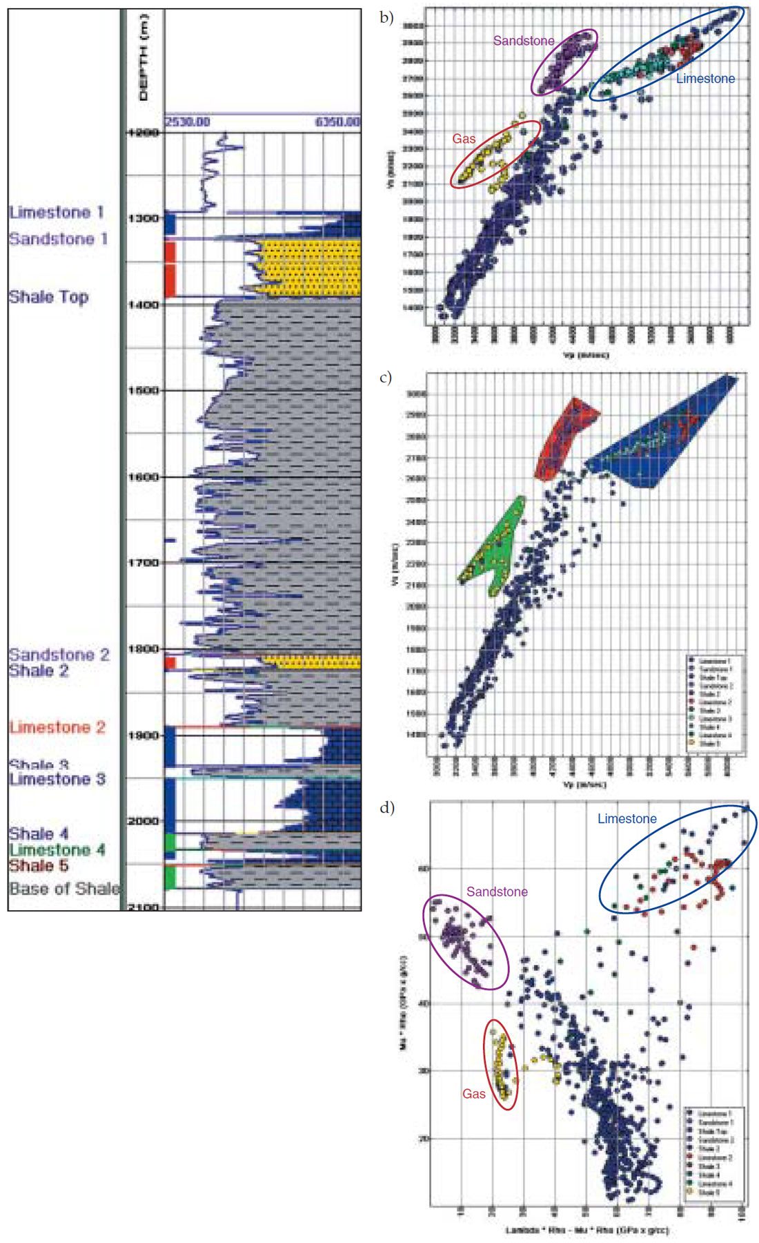
Figure 1(b): Cross-plot of Vp vs Vs The different formation tops are seen marked on the curves and correspond to at least four limestone layers, two sandstone layers and four shale layers.
Figure 1(c): Cross-plot of Vp vs Vs with polygons around individual clusters highlighting the range of points on the logs seen in Fig.1(a).
Figure 1(d): Cross-plot of Lambda-Rho vs Mu-Rho shows better separation of clusters. Lambda-Rho is a sensitive indicator of water vs gas saturation and Mu-Rho is used to help pure rock fabric or lithology.
As mentioned earlier, convincing cluster patterns can be seen in the derived elastic parameter cross-plot space. All such crossplots can be generated on the fly. Fig. 1(d) shows a cross-plot comparison of LambdaRho versus MuRho. LambdaRho is a sensitive indicator of water vs gas saturation and MuRho is used to help pure rock fabric or lithology. Clearly, the different clusters are more separated in this crossplot as compared with the Vp versus Vs crossplot.
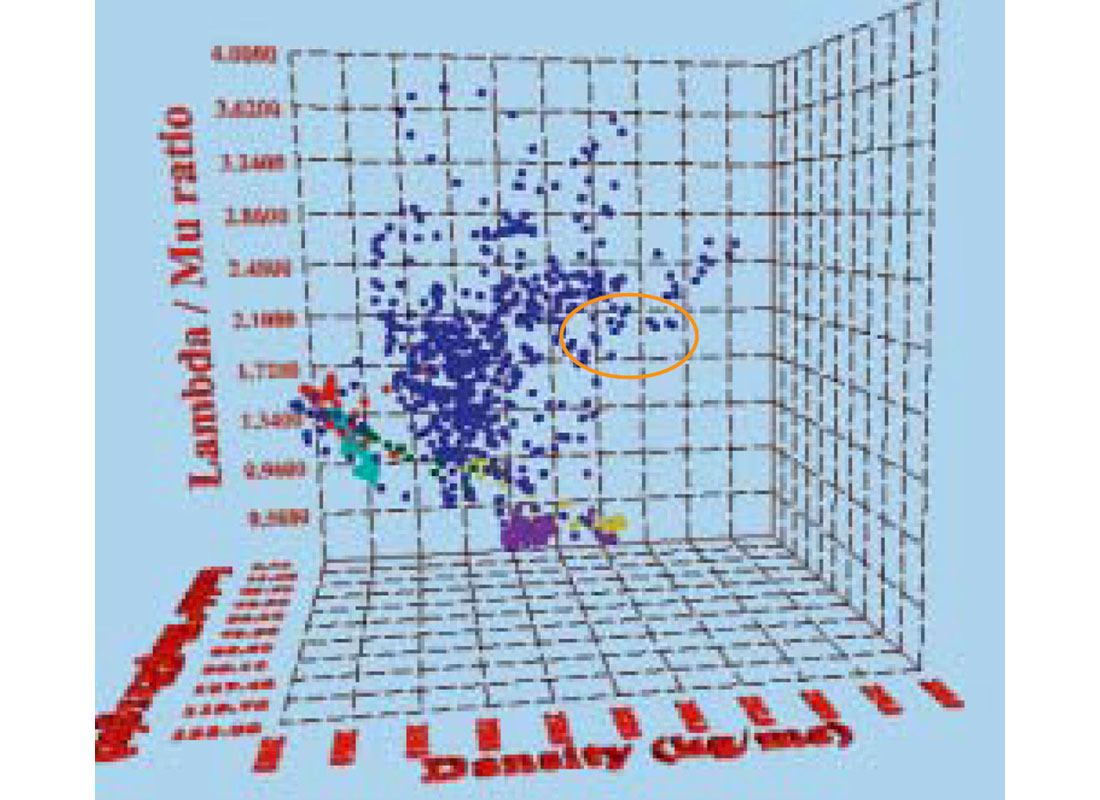
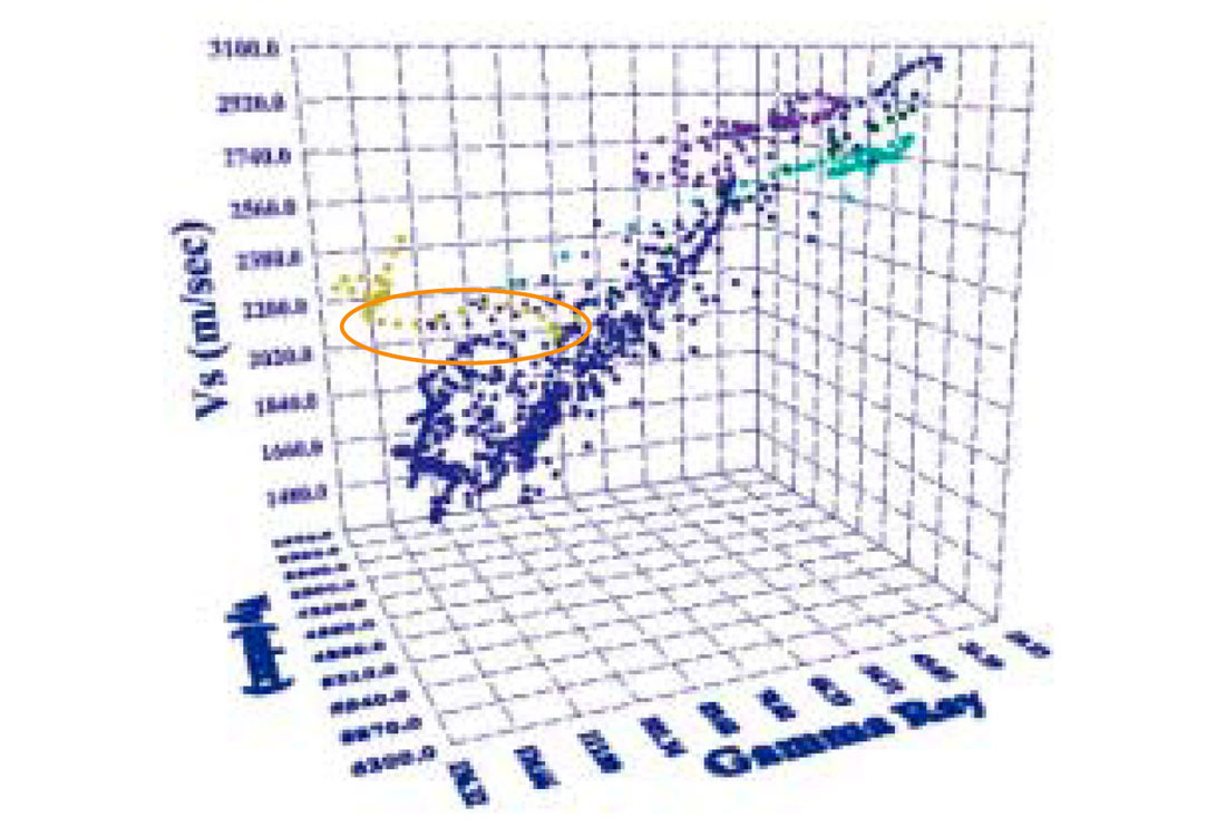
It is possible to add a third dimension to any of these crossplots by choosing, for example either a density axis, a porosity axis or a ‘Gamma Ray’ axis. Figures 2 (a) and (b) shows two 3-D crossplots, one with density and the other with gamma ray. Two useful observations emerge:
1. Looking at the LambdaRho versus Lambda / Mu crossplot, the carbonate cluster is seen comprising the four different layers of limestone. However, as the 3-D crossplot cube is turned about the vertical axis, it is noticed that the density of limestone layer 1 is not high as for the other layers and also there is a variation in density in this layer. This could imply that limestone layer 1 interpreted as one layer could possibly be a combination of two sublayers with different densities (indication to this effect seen in Fig.1(a)).
2. The curved layer one sees linked to the gas producing Barnett Shale cluster may not represent a part of it; as we see in Fig.2(b), while the linear trend is seen associated with high gamma ray values, the curved sliver shows a gradual variation in these values which extend over at least 40 API units (indicated with a red bracket).
Interactively examining all the available and derived curves in 3-D crossplot space enables the interpreter to conveniently understand the lithological layering in the subsurface and assess the hydrocarbon-bearing zones or key lithologies better.
Example 2
In gas hydrate studies, the electrical resistivity and sonic logs are usually used for their identification. In contrast to water-saturated sediments, gas-hydrate-bearing sediments exhibit anomalously high electrical resistivities and high acoustic velocities. The solid nature of gas hydrates makes the porous rock more supportive for seismic wave propagation (particularly P-wave propagation). Therefore, the compressional velocity in gashydrate-bearing sediments is usually several times higher than that in gas-bearing sediments. Such gas-bearing zones appear as anomalous low velocity zones. Consequently, at the base of the gas-hydrate stability zone, which marks the contact between gashydrate and free-gas bearing sediments, the sonic log, is characterized by a distinct drop in acoustic velocity from the gas-hydrate bearing section above into the underlying free-gasbearing interval.
The Mallik 2L-38 gas hydrate research well was drilled by JAPEX/JNOX/GSC in early 1998 to a depth of 1150 m (Dallimore et al 1999). The base of the methane hydrate stability zone, predicted from borehole temperature surveys, is at a depth of 1100 m. Borehole electrical resistivity and acoustic velocity (both P and S) logs confirm the occurrences of insitu gas hydrates between 888.84 and 1102.2 m. Based on the core analysis and logged gas hydrate occurrences in Mallik 2L-38, deep electrical resistivity measurements range from 10 to 50 ohm-m., compressional wave velocity range from 2.5 to 3.6 km/s and shear wave velocity from 1.1 to 2.0 km/s. In 3-D crossplot space, by choosing any of these 3 parameters, it is possible to visualize the anomalous cluster patterns and make the necessary inferences (Fig.3(a) to (e)). The hydrate layers indicate large resistivities (depending on their saturation) and smaller ‘gamma ray’ values (depending on the lithology).
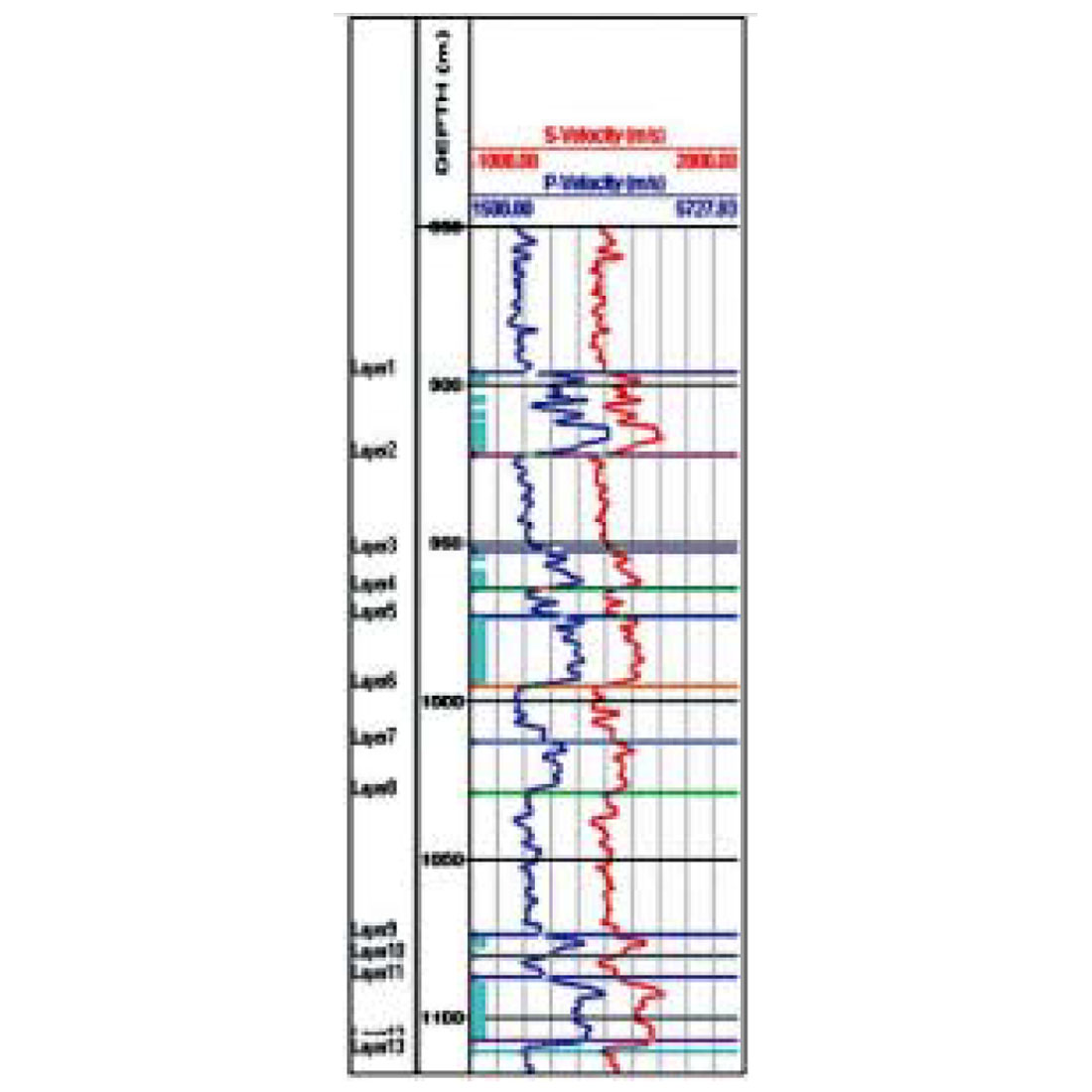
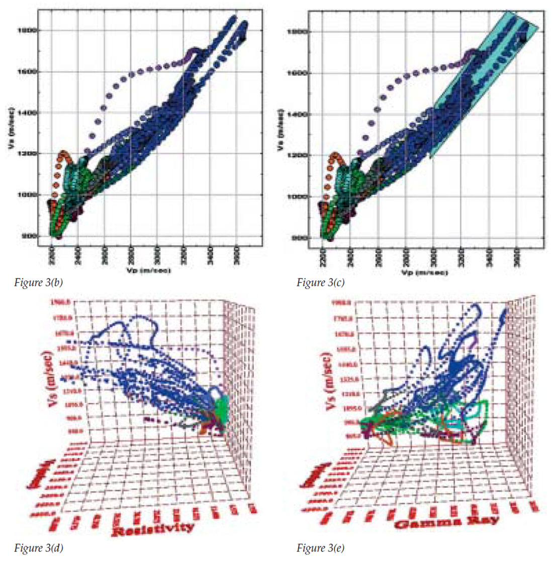
Figure 3(c) Cross-plot of Vp versus Vs with a polygon enclosing the points corresponding to hydrates. Log zones from where the enclosed points originated can be seen on the log curves in Figure 3(a).
Figure 3(d): 3D cross-plot of Vp-Vs- Resistivity. Notice that the blue clusters exhibit a variation in the resistivites of the hydrates depending on their saturation.
Figure 3(e): 3D cross-plot of Vp-Vs- Gamma Ray. Notice that the blue clusters exhibit a variation in the gamma ray values of the hydrates depending on the lithology.
Interactive 3-D AVO Attribute Crossplotting
Interactive 3-D crossplotting is computationally intensive. To get a feel for this computation, a 100 sq.km. area with a 500 ms time window at 2 ms sample rate and a square bin of 25 m will generate 40 million pairs. Loading a 3-D volume with 200 inline and 200 crosslines, 500 ms segmented window, 2 ms sample interval and a square bin of 25 m, brings in 10 million pairs. While it is possible to load this bulk of data, the quantity of data coming in could be overwhelming in that the high density of individual points, due to their opacity, may mask the extraction of meaningful information from the clusters that the anomalies entail. It is of course convenient to load sub-volumes that encompass the anomalies of interest, but for a manageable data set to be visualized, suitable decimation (every alternate inline or cross line or any other increment) may also be required apart from segmentation (suitable time window).
Figure 4 shows an example from a producing Cretaceous-aged gas field in southern Alberta. At least three sand-bearing channels can be interpreted on a composite plot where high amplitude envelope values are overlayed on a coherence slice (Figure 4(a)). This has independently been confirmed by Lambda-Rho and Mu- Rho analysis (Pruden 2002). Fig.4(b) shows a 3-D crossplot for the anomaly on the right in Figure 4(a). Twenty one complete inlines (10 on each of the blue line shown in Figure 4(a)) have been selected and 200 ms of the data, comprising the broad zone of interest). Lambda-Rho and Mu-Rho volumes have been used for generating this cross-plot. Lambda-Rho, Mu-Rho and Inlines are seen on the three axes in Figure 4(b). The cluster of points are shaded in at least 3 different colours – bright red, purple and blue. Clearly, the red cluster of points (highlighted) within the ring corresponds to the anomaly. As the 3-D crossplot is turned to one side, the bright red cluster is seen to extend over a certain patch of inlines and this areal spread of the red cluster indicates the extent of the anomaly.
While this 3-D cross-plot gives a visual sense about the areal spread of the anomaly in Lambda-Rho vs Mu-Rho cross-plot space, one could argue that it is essentially a series of 2-D Lambda-Rho vs Mu-Rho cross-plots stacked together, one for each of the 21 inlines considered. This prompts us to think of choosing three different parameters on the three axes of the 3-D cross plot. The combination of parameters chosen should then enable a convenient and meaningful deciphering of anomalous clusters in 3-D cross-plot space. Lambda-Rho, Mu-Rho and fluid stack could be one such combination. Fluid stack highlights zones where the P-reflectivity is different from S-reflectivity. While these two will be pretty much the same, for gas bearing zones the P-reflectivity will be different (lower) from the S-reflectivity and an indicator that displays these differences is interesting. A gas sand, for example, would exhibit low values of Lambda-Rho, high values of Mu-Rho and negative values of fluid stack.
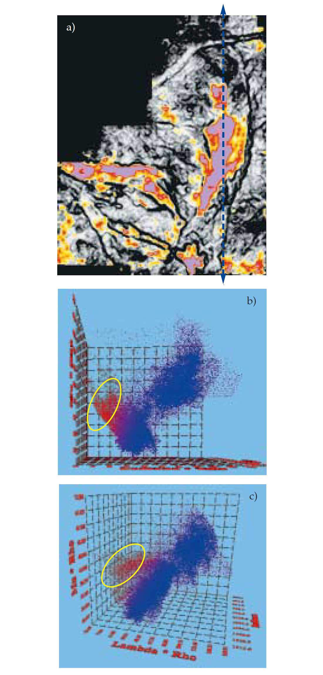
Figure 5 shows these three indicators cross-plotted for a gas anomaly, (Lambda-Rho on the x-axis, Mu-Rho on the y-axis and fluid stack on the z-axis). Figure 5(a) shows a time slice from a Lambda-Rho volume and the gas anomaly is indicated by the blue patch. A polygon (red) is drawn to select the live data points on the time slice that can be brought into the crossplot. The red cluster of points seen in Figure 5(b) comes from 5 time slices that have been selected for the purpose. It is possible to narrow down on a given anomalous region by drawing different coloured polygons, looking at the clusters they light up in 3-D cross plot in that colour. As the crossplot is turned towards the left on the vertical axis, the fluid stack shows the expected negative values for the gas sand. It is possible that the clusters of points coming from outside the anomaly clutter the crossplot and may mask the points coming from the anomaly. A selection of points coming from any polygon can be incorporated into the software to allow the desired set of points to be displayed in the cross plot. As seen here only the points coming from the purple polygon can be seen in Figure 5(e).
(a) Polygons selected on a time slice from the Lambda-Rho volume. The red polygon encompasses the entire are being analyzed.
(b) Points within the red polygon only are seen in the 3D cross plot.
(c) Points within the red, yellow and purple polygons show up as different clusters. The gas anomaly indicated by blue color on time slice and enclosed by purple polygon is seen showing up as negative values for fluid stack, a prospective cluster.
(d) 3D cross plot seen from the fluid stack side of the 3D cross plot.
(e) 3D cross plot seen from the fluid stack side of the 3D cross plot with points only from the purple polygon.
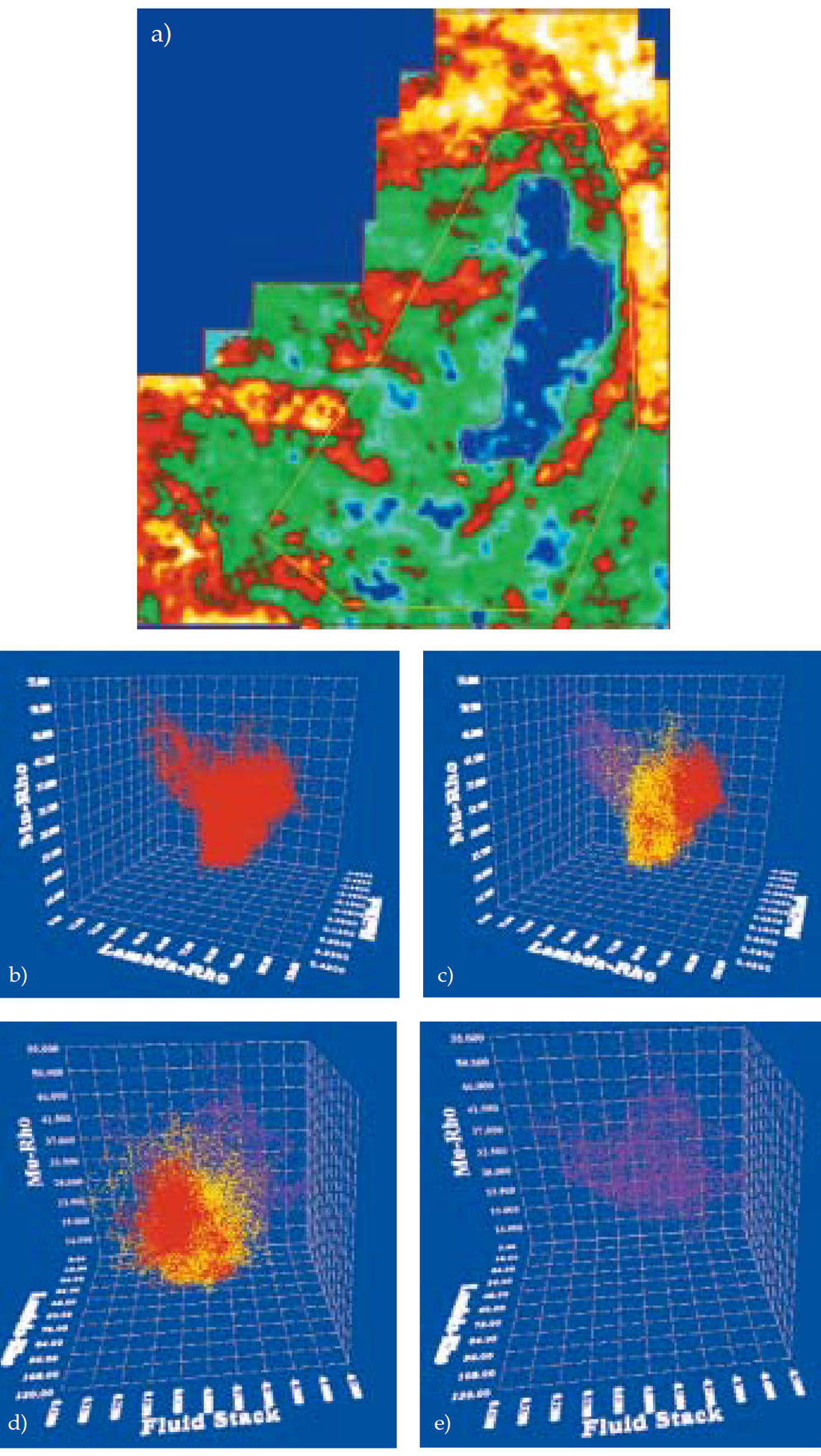
Similarly, Figure 6 shows LambdaRho - Lambda/Mu - Fluid stack 3-D cross plot. In Figure 6(a), corresponding to the prospective anomaly, a yellow polygon drawn within a red polygon shows low values of LambdaRho and low values of Lambda/Mu (not shown), which are expected of a gas sand. Figures 6(b) and (c) show the spread of these low values (yellow) indicating negative values for fluid stack.
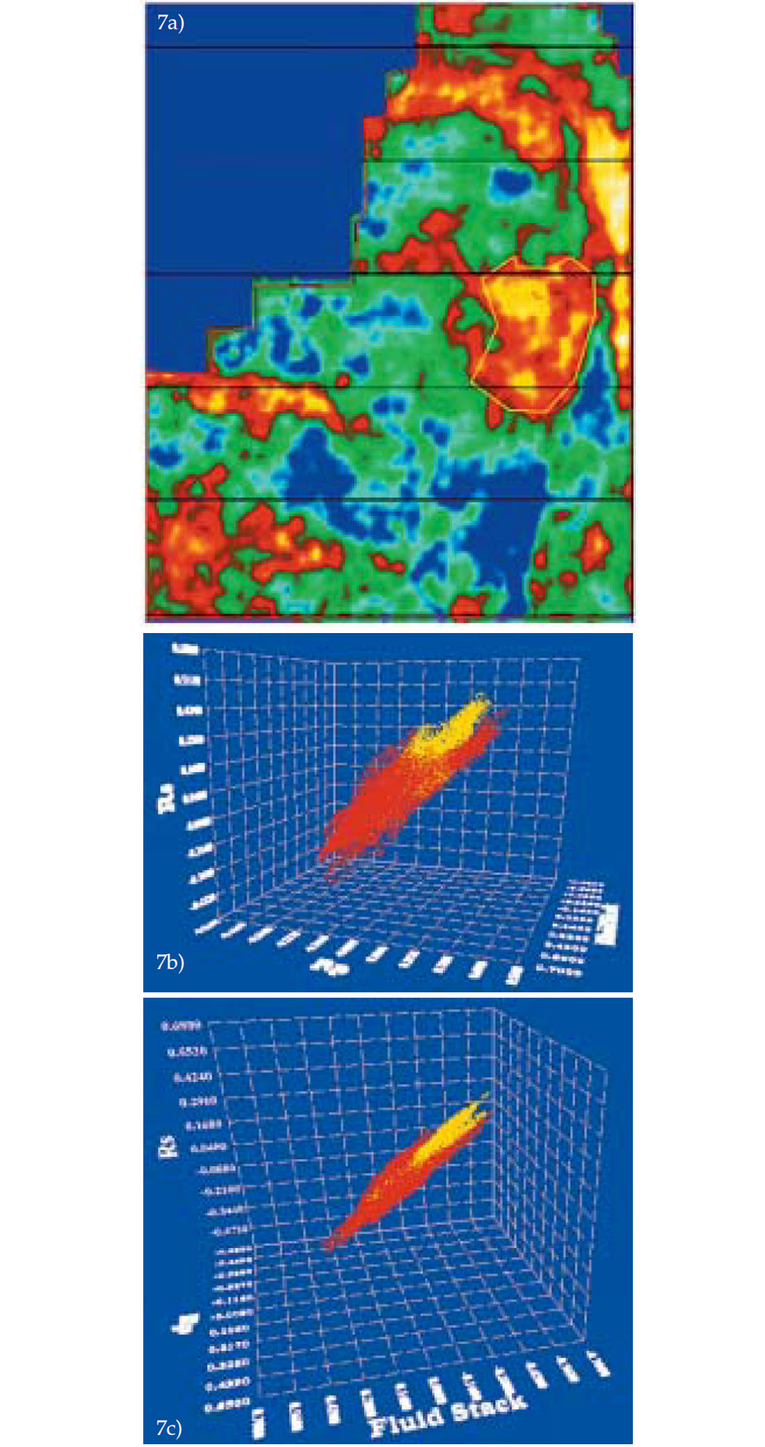
Figure 7 shows a time slice from the P-reflectivity (Rp) volume for the same data set used in Figures 4, 5 and 6. A yellow polygon is shown marking the anomaly. The same polygon is assigned to the S-Reflectivity (Rs) and fluid stack time slices. On the 3-D cross plot with Rp, Rs and fluid stack on the three axes, the yellow polygon lights up a yellow cluster in a red background cluster. As the cube is turned, the fluid stack indicates these negative yellow values corresponding to the anomaly.
Though not included in this analysis, an ideal combination of the three attributes would be Lambda–Mu–Density. Distinction between highly porous, gassy oil versus lower porosity could be made on the Lambda axis, sand shale and silt clusters could be distinguished on the Mu axis and porosity could be visualized on the density axis. For appropriate data, such a 3-D crossplot would be very useful.
Pre-stack application of HFR
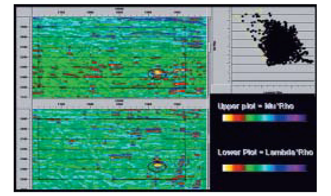
High Frequency Restoration (HFR) is a procedure consisting of the determination of decay in frequency from downgoing VSP first arrivals from successive depth levels, and then applying the inverse decay function to surface seismic data (Chopra et al, 2003). Application of HFR to pre-stack seismic data is very effective and useful for AVO analysis. A zero offset VSP is used to determine the attenuation in terms of a set of time-variant HFR filters, and applied to the seismic gathers. This enhances the frequency content of the data going into AVO/LMR analysis and is useful for thin bed analysis. Figure 8(a) shows a cross-plot of LambdaRho versus MuRho for the two sections shown therein from South China Sea. A polygon (in yellow) encloses the cluster of points that look prospective and highlights the anomaly (indicated) on the two sections. After application of HFR on the gathers and putting them through the same AVO/LMR processing the sections shown in Figure 8(b) are obtained. Notice, the cluster of prospective points seem to be forming a more definitive pattern (and still highlights the same anomaly) which could be quite meaningful when looking for thin bed anomalies.

Conclusions
With any three attributes seen together on a 3-D cross plot, it is possible to look through more data quickly and conveniently. It is not just a planar 2-D view that one usually looks at, rather the disposition of individual clusters in a 3-D cube which can be turned in any direction to get a detailed understanding of their arrangement or distribution.
The 3-D cross-plotting visualization of LMR (Lambda –Mu–Rho) attributes enables the display of cluster distribution corresponding to different lithologies, when properly colour-coded. Such analyses are not so revealing on 2-D cross plots. As stated earlier, for getting good results, the range and limits of data to be cross plotted need to be judiciously decided.
AVO interpretation based on 3-D cross-plotting is more insightful, reliable, accurate and therefore more useful.
Cross-plotting for AVO analysis done on data with HFR provides more meaningful patterns to be interpreted for anomalies.

Acknowledgements
We gratefully acknowledge the data courtesy extended to us by Kicking Horse Resources Ltd. Calgary. We thank Doug Pruden, GEDCO, Calgary, for the initial interpretation carried out on the data, Jan Dewar for her valuable comments and suggestions and Joanne Lanteigne for formatting some of the images. Our special thanks go to Vasudhaven Sudhakar for encouraging this work and to Core Laboratories for permission to publish this paper.
Coherence Cube & HFR are trademarks of Core Laboratories.


Join the Conversation
Interested in starting, or contributing to a conversation about an article or issue of the RECORDER? Join our CSEG LinkedIn Group.
Share This Article