Abstract
Migration is an important stage in seismic imaging that focuses the recorded seismic data and generates a true structural image of the subsurface. In complex fault and fold thrust belts with rough topography, migration is difficult owing to lateral velocity changes and also very steep dips. The geometry of acquisition in complex geological situations with rough topography is seldom regular so Kirchhoff prestack depth migration is the method of choice. To obtain a better image from two complicated fault and folded structures in the Iranian Zagros fold and thrust belt, Kirchhoff prestack depth migration methods have been applied and the effects of different Green functions have been investigated. The complexities are both at the near surface (effects of variation in elevation) and deep in the subsurface (intense folding and faulting, lateral velocity variation, lithological changes, and thick salt layers). The travel time computation methods have a great impact on the result of Kirchhoff prestack depth migration in complex geological cases. Four different traveltime computation methods have been tested: ray tracing with minimum arrival in a rectangular coordinate system, ray tracing with shortest path in a rectangular coordinate system, eikonal solver, and ray tracing of first arrival in a spherical coordinate system. By constraining the single arrival Kirchhoff prestack depth migration with hard geologic information including detailed seismic interpretation (controlled by more than 90 wells) we achieved results that are significantly more useable than those from unconstrained Kirchhoff prestack depth migration. The spherical coordinate system for travel time calculation gives better results than a rectangular coordinate system. Around the flanks of folds with very steep limbs selecting the single arrival with shortest path (head wave killer) rather than minimum arrival time gives better focusing.
Introduction
Migration is an important stage in seismic imaging that focuses the recorded seismic data and generates a true structural image from the subsurface. It removes the effect of seismic wave propagation (e.g. diffraction from sharp edges) from data, therefore seismic events move towards their correct subsurface positions. There are several migration methods available for imaging different types of geological situations. Making the best choice needs an understanding of the various techniques. In complex fault and fold thrust belts with rough topography, migration is difficult owing to lateral velocity changes and also very steep dips. Reflection events are not hyperbolic and so the stacking process does not work well. When there is lateral variation in the velocity model the RMS velocity used in time migration fails to describe the geometry of the diffraction. Therefore prestack depth migration is the state of the art solution for seismic imaging in such situations (e.g. Yan, et al., 2001).
The geometry of acquisition in complex geological situations with rough topography is seldom regular so Kirchhoff prestack depth migration is the method of choice. This method is less sensitive to irregular spatial sampling of 3D prestack data than other methods. It also has the possibility of target oriented processing and input/output flexibility and computation efficiency (Audebert, et al., 1997). In structurally complicated areas, seismic imaging is difficult and needs to involve interpretation (Gray, 2000). By constraining the Kirchhoff prestack depth migration with hard geological information, one can achieve results that are significantly more useable than those from unconstrained Kirchhoff prestack depth migration. Kirchhoff prestack depth migration is efficient in providing target-oriented outputs for selected data subsets. Another advantage of the Kirchhoff migration method is its flexibility in handling irregular topographic surfaces, since it does not require a flat datum like the extrapolation or direct wave equation based methods.
To obtain a better image from two complicated faulted anticlines in the Iranian Zagros fold and thrust belt, Kirchhoff prestack depth migration methods have been applied and the effects of different Green functions have been investigated. Any correct depth imaging requires a correct interval velocity model. The interval velocity model used in this migration test has been prepared using an initial velocity model derived from prestack time migration processing and later modified and updated by using hybrid depth tomography (both grid based and layer based) and constrained by geological information including well data and seismic interpretation. The Exploration Directorate of the National Iranian Oil Company provided the Data.
Kirchhoff Pre Stack Depth Migration Method
The Kirchhoff integral that is used for data extrapolation and migration (Schneider, 1978, Wiggins, 1984, Bleistein and Gray, 2000, French, 1975, Audebert, et al., 1997, Docherty, 1991) is based on Green’s theorem (Morese and Feshbach, 1953) and an integral solution of the wave equation. 3D prestack seismic data are recorded on separate sets of surface points. In practice the approximate Kirchhoff integral is (Biondi, 2004):

where the image I(r), defined in a three-dimensional space r = ( x, y, z ), is equal to the summation of data values D ( t , m , h )evaluated at the time tD( r, m, h) and weighted by an appropriate factor W( r, m, h) for amplitude. mi and hi are midpoint and offset positions. The procedure is based on diffraction summation. The summation surfaces are the basis of the Kirchhoff migration and in terms of physical interpretation they are diffraction surfaces for point scatterers located in the subsurface. The diffraction from an isolated point scatterer in the earth’s subsurface would create events with the same shape as the summation surfaces. The summation domain is limited to a region at the m or midpoint plane. The image point is located at the centre of the summation domain. The summation subscript i indicates the finite number of seismic recorded traces. tD is the travel time from the source point to imaging point and from the imaging point back to the receiver (tD =ts+ tr ). In complex situations such as fold thrust belts the time delay function between the source-receiver points and the imaging point does not follow simple analytical relationships such as (Biondi, 2004):

As a result the summation surfaces have more complex geometry.
There are several travel time computation methods for such complex cases. All methods are based on a high frequency approximation of the wave equation (eikonal equation) (Bleistein, 1984, Bleistein, et al., 2000, Cerveny, 2001). The equation has usually been solved by ray tracing methods (Cerveny, 2001), which solves the eikonal equation along its characteristics.
The summation indicated in equation (1) is numerically computed as a loop over each image point and sums the contributions of all input traces that are within the migration aperture. Kirchhoff prestack depth migration uses the actual raypath from every source to every receiver. This raypath is used to construct the diffraction surface. The migration of a seismic section is achieved by collapsing each diffraction hyperbola to its origin (apex). In practice, each offset plane is first migrated separately and then, all offsets are summed together to generate the stacked migrated image. Therefore, the Kirchhoff prestack depth migration is performed in two steps. First summing data points with equal offsets and then summing along offsets.
Input Data Set
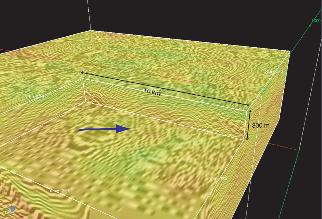
The 3D seismic dataset that has been used in this study was acquired from two producing oil fields located in the Iranian Zagros fold belt (Parsi at north and Karanj at south) (figure 1). The acquisition parameters are given in table 1. The topography of the survey area varies between 350m to 1200m. Topographic variations cause irregular distribution of source and receiver points. An example of such a case is given in figure 2. The black points are the shot point locations. The planned source line interval is 400m while there are situations with more than 800m source line interval. This irregularity of data distribution imposes a major limitation on any prestack imaging method. Kirchhoff pre stack depth migration has flexibility at least for irregular spatial sampling and also topographic variations.

| Table 1. Acquisition parameters of Parsi and Karanj 3D survey | ||
| Bin size | 20mx40m | |
| Total number of bins | 999060 | |
| Receiver line interval | 320m | |
| Source line interval | 400m | |
| Total number of recorded points | 24809 | |
| Patch | 6 lines each with 160 channels | |
| Nominal stacking fold | 24 | |
| Maximum offset | 3413m | |
| Aspect ratio | 0.39 | |
| Source type | Dynamite | |
The pre-processing procedure is important since it can improve the quality of input data for seismic imaging (both velocity analysis and migration). The main goal of pre-processing is to suppress the noise as much as possible while keeping signals untouched. The main steps of pre-processing applied on the input data before seismic depth imaging are given in table 2 (CGG, 2003).

| Table 2. pre-processing parameters of Parsi and Karanj 3D survey |
| Trace geometry updating control |
| Spherical divergence correction. Each sample is multiplied by T x V2 |
| Instrument compensation |
| Primary static application to floating datum plane (FDP)Computation from the 3D near-surface model derived from upholes Correction velocity: 3000 m/s Datum elevation 1300 m |
| 3D FK conical filter (FKx-Ky) in Cross spread domain– velocity cut-off: 2600 m/s – attenuation: 24 dB |
| Additional gain versus time (3 dB per second) |
| Gain versus offset |
| Automatic editing of noisy traces Statistical editing based on average amplitude comparison |
| 3D surface consistent amplitude correction (source and receiver)computed in window 500 – 2000 ms |
| 3D surface consistent spiking deconvolution (zero phase output) |
An amplitude spectrum of the pre-processed time gathers showed a high noise level particularly in low fold areas. Figure 3a shows an example of noisy gathers. The anomalous spikes in the prestack time gathers will generate noise in the migration process. In order to suppress the remaining noise some more preprocessing has been done in time. The suppression of coherent noise is difficult since it may lead to the loss of part of the signal as well. The processing steps have been applied before running Kirchhoff prestack depth migration as given in table 3.

| Table 3. Additional noise removal |
| Specific frequency noise removal (mono-frequency attenuation) |
| Inner (X, T; 0, 800; 400,1300; 450,5000) and outer mute (X, T; 0,0; 3200,700). |
| Trace scaling with 50 percent overlapping |
| Table 3. Additional noise removal |
| Band pass frequency filter (5,15,60,75 Hz for T0-T1000 and 5,15,40,60Hz for T2500-T6000) |
| Specific frequency noise removal (mono-frequency attenuation) |
| Inner (X, T; 0, 800; 400,1300; 450,5000) and outer mute (X, T; 0,0; 3200,700). |
| Trace scaling with 50 percent overlapping |
Sources Of Complexity
The sources of complexity in the studied area are typical of the complexities of mountainous areas of fold belts.
First of all, the near surface problems cause data to be distorted. These include the effects of variation in elevation, near-surface low-velocity-layer (weathering layer) thickness, weathering velocity, and the reference to a datum.
The complexities below the near surface section can be divided into the two main categories: structure dependent and structure independent. The main producing interval is the Asmari formation that consists of carbonate rock. There is a clear difference in structural style between the horizons above this formation (post- Asmari interval) and the horizons below it (pre-Asmari interval). The lower part of the post-Asmari interval is dominated by large thickness variation over short distances, internal faulting, and folding. This thickness variation causes rapid lateral velocity variation. The same interval (post-Asmari) consists of several layers of salt and anhydrite. The thickness of the salt intervals changes rapidly due to compression. There are also rapid lateral changes in rock types (due to the nature of deposition of these sediments) that make this formation complex in terms of rock properties. The salt layers of the overburden also generate illumination problems for the pre-Asmari interval. The complexities in the pre-Asmari interval are partly related to structural complications in the interval itself and partly due to the problems generated by the post-Asmari depth interval.
In the Zagros fold and thrust belt in general and in the Parsi and Karanj oil fields in particular the flanks of the anticlines in pre-Asmari interval are usually asymmetric and one of the flanks (the south flank in many cases) is steeper than the other. Therefore imaging the steep flanks of the folds in Zagros fold and thrust belt was a difficult task for exploration seismologists for years. The problem of imaging the steep flanks became the subject of discussion among geophysicists and geologists. Geophysicists put thrusts in the flank of the folds to describe the geometry while geologists believed in overturned limbs of the folds (Motiei, 1995). The reliance on structural styles is necessary in view of the fact that the quality of the seismic images of fold and thrust structures is poor (Lingrey, 1991).
The next main problem is the complex internal structure of the folds in the pre-Asmari interval. Conventional seismic images give a rough picture from the structural configuration of deeper levels in the pre-Asmari interval. This picture is not clear enough to draw the correct geometry of the structures. As a result of this ambiguity the wells drilled at apparently undisturbed parts of the anticlines (mainly crest of the folds) encountered structural complexity at deeper levels. As stated before in such cases any attempts to interpret the poor quality seismic profiles were based mainly on the structural styles not on what can be directly extracted from the seismic image itself. The final problem of the pre-Asmari interval is the lithology variation in rock units. The main constituent of pre-Asmari interval is carbonate and some intervening shale intervals. Velocity variation in carbonates is not depth dependent but it is dependent on depositional environment (Anselmetti and Eberli, 2001). Velocity inversion also occurs in shale units bound between carbonate units.
Kirchhoff Prestack Depth Migration Results
The Kirchhoff 3D prestack depth migration is performed in two steps. In the first step travel times are calculated and then, at the second step migration is performed. Interval velocity analysis and prestack depth migration are two main parts of seismic depth imaging that are closely linked together. In order to have well focused data and produce a correct subsurface image, migration must be done with adequate information on propagation velocity. The input interval velocity model used for Kirchhoff prestack depth migration is the same and has been prepared with an integrated model-based migration velocity analysis procedure. Grid-based and interface-based depth tomography of common image input gathers have been applied with seismic interpretation and well-derived information to constrain the velocity estimation procedure. Relevant a priori information has been proposed for each stage to constrain the velocity analysis. The migration velocity analysis starts from regional updates with structural framework reconstruction and ends up in a detailed velocity model that is consistent with the complex geometry as well as with the rock types.
The travel time computation methods have a great impact on the result of Kirchhoff prestack depth migration in complex geological cases. Two different algorithms have been tested. The first one is based on ray tracing and the second solving the eikonal equation. In the first algorithm the actual ray path between two points has been tracked through the complex velocity model. The traveltime along the raypath is computed by integrating the velocity function along the ray. In the second method instead of tracing the rays, traveltimes are calculated from the equation that describes the change in traveltime as a function of location for a given velocity function. The coordinate system of the velocity and data grid is an important factor. Two types of coordinate system have been used: rectangular and spherical. The spherical grid is closer to the geometry of a real wavefront and provides a better image. The following four traveltime computation methods have been tested:
- Ray tracing of a single arrival with minimum traveltime in a rectangular coordinate system: This travel time computation in a rectangular grid is based on Fermat’s principle. The actual ray chosen from several rays connecting source and receiver points is the one with minimum travel time (Meshbey, et al., 1996). The minimum travel time assumption is applied to find the travel time of the selected ray for each depth interval and then the search in the following intervals is limited to a region around that selected ray. The accuracy of travel time computation is dependent on the thickness of the depth intervals chosen for ray tracing, and with large intervals the accuracy will decrease. In complex situations where the velocity varies both laterally and vertically it is better to select finer depth intervals for travel time computation. This method is the fastest of the four tested methods.
- Ray tracing of a single arrival with shortest path in a rectangular coordinate system: In most cases the direct ray is required by Kirchhoff migration. Sometimes the head wave arrives first and the direct ray is the one with shortest path and not minimum time. The problem of seismic depth imaging in complex media is manifested by the existence of triplications in ray tracing (Xu, et al., 1999) and as result multivalued travel times that put a limitation on single arrival travel time solvers (Geoltrain and Brac, 1993, Operto, et al., 2000, Xu and Lambare, 2004). Geoltrain and Brac (1993) have shown the failure of using first arrival travel time in complex media. This failure is due to the fact that both secondary arrivals and associated amplitudes of those arrivals are not taken into account. The amplitude will be better preserved if the strongest arrival selected in the migration (Audebert, et al., 1997, Thierry, et al., 1999) is chosen. The best solution is to use the travel times of multiple arrivals (total ray-field information) and weight them by their amplitudes depending on the geometrical spreading and ray angles. This is a difficult task and is highly sensitive to errors in the velocity model. However using a single strongest arrival improves the migration (Thierry, et al., 1999, Xu, et al., 1999, Operto et. al., 2000). The use of the most energetic arrival is a reasonable alternative solution to multivalued travel time computation. The ray tracing method used in this study is an upward shooting approach (Meshbey, et al., 1996) that makes it possible to select the shortest path or the most energetic arrival.
- Eikonal-equation solver in a spherical coordinate system: In this method travel times are computed by solving the eikonal equation. Actually the travel time function is a solution to the eikonal equation (Cerveny, 2001)

- Ray tracing of first arrival in a spherical coordinate system: The spherical coordinate system in ray tracing is more time consuming than a Cartesian coordinate system but is closer to the real wavefront. The requirement on CPU time in a 3D seismic depth imaging is important and is one of the parameters controlling the selection of any imaging method.
The same interval velocity model has been used for all travel time solutions and the migration aperture for all migration tests was 300 inlines and 300 crosslines. In complex situations with steep dips, the Kirchhoff migration for a given input seismic trace spacing is aliased. This generated some artefacts in the migrated image especially in the shallow section. Anti-alias filters are used to avoid generation of these artefacts. It works as high-cut filtering of lower frequencies of input data at larger summation angles. By using this filter migration can be performed with large apertures without degradation of the data by aliasing noise.
The quality of images from the steep flanks of the structures in the pre-Asmari interval, correct geometry of thrust surfaces, and internal faulting and folding of the post- Asmari interval are some of the elements that can be used to evaluate the quality of prestack depth imaging results.
Figure 4a shows the migration result for the first travel time computation method. This is the fastest travel time computation method and only the first arrival (minimum traveltime) has been taken into account. The steep flank of the structure (southwest limb) is missing completely. The upper-most picked reflector is the top of pre- Asmari interval. The two reflectors picked in the southwest part of the section are the possible location for another deep anticline. But the events are not coherent enough to draw the complete picture of this deep small anticline. The geometry of the thrust fault between two anticlines is not clear enough. Actually this poor quality image causes an incomplete if not wrong definition of the structure. Interpretation in such cases relies more on pre-existing knowledge of the structural style in the area, that itself comes partly from the study of seismic profiles.

Figure 4b shows the results of second traveltime computation method on the same inline as figure 4a. The selected single arrival is the one with minimum path (shortest path) rather than minimum travel time. The top Asmari reflector extends more towards the southwest (the upper green picked horizon to the right of the section). The structure located at the left side that was not clear in the previous migration is better imaged. This result shows that for certain structures such as the steep flanks that have strong lateral velocity variations in the post-Asmari depth interval, using the minimum travel time assumption is not right. The strongest arrival in this part of the structure is the one with shortest path, which passes through a low velocity interval right above the Asmari reflector in the post-Asmari depth interval. In these cases selection of the first arrival instead of the shortest path gives a shorter travel time and as a result the reflectors are pushed down in the migrated image. The reflectors focusing in the deeper part of the pre-Asmari depth interval (for example the lower picked horizon to the right of the section in figure 4b) have also been enhanced with respect to the previous migration.

Another example of the difference between minimum travel time and shortest path is given in figure 5a and b. There are significant improvements in the focusing and image quality in figure 5b. The arrow shows the location of the deep structure. The thick overburden sequences with strong heterogeneity make the correct imaging of this deep anticline very difficult. The improvement shown in figure 5b is remarkable. The structure can be picked with great confidence. The southern flank of the structure to northeast is also imaged well with the shortest path travel time computation method (figure 5b). There are three structures shown in figure 5b by characters A (southern structure), B (middle structure) and C (northern structure). The reflector packages above middle structure in figure 5b (the yellow arrow) are an excellent well-focused reflector package from the post-Asmari interval. The purple arrow in figure 5b shows the position of a thrust plane where southwest dipping beds are juxtaposed with northeast dipping beds. Figure 6a and b show the comparison of ray tracing based on shortest path travel time solution in rectangular coordinate system (method 2) with the eikonal solver for travel time computation (method 3). The picked horizons are drawn simply to show the reflector continuity in the northern and middle structure. The upper green horizon is close to the top of pre-Asmari depth interval. As it has been stated earlier the poor quality of the images from the flanks led to two different thoughts among geologists and geophysicists (Motiei, 1995). Figure 6b shows that the southern flank of northern structure at the location of this inline is continuous and there is no evidence of reverse faulting in the flank. The thrust fault between the northern structure and the middle structure is also well focussed.

The results of the ray tracing in a spherical coordinate system (method 4) show better focusing and imaging compared to the 3 previous methods. Figure 7a and b show a comparison between the eikonal solver (method 3) and the ray tracing in spherical coordinate system (method 4). The southern flank of northern structure in figure 7b is extended more than in figure 7a. The arrows at the right side of figure 7a and b show the improved imaging/focusing in the post-Asmari (overburden) interval with ray tracing in a spherical coordinate system. The chosen coordinate system strongly affects the travel time computation.


Figure 8 is another inline from a very complex part of the dataset. Rapid thickness variation in the post-Asmari interval, large structural elevation difference in pre-Asmari depth interval from northern structure to the southern one and a significant ambiguity in the middle structure are some of the imaging problems. The improvements achieved in focusing and image quality by Kirchhoff prestack depth migration with ray tracing in spherical coordinate system is remarkable. A general interpretation has been done (figure 9) to show the improvements that have been achieved by this migration method. The inline shown in figure 9 includes a wider area than the inlines shown in figures 8a and b. The structure to the right is the northern structure. The position of the reflectors in the picked area is confirmed with the well information. The transition from the northern structure to the middle one (structure B in figure 9) defines the location of a thrust fault as is shown by the arrow in the figure 9. The structural configuration of the southern structure (structure A in figure 9) is also clearly imaged. Figure 10 is a 3D slice of the migrated data using the fourth method and it shows the clear image from the flanks of the northern structure both in cross section and depth slice view.

In complex situations where the seismic migration objectives are to obtain a geologically consistent image, seismic imaging is essentially interpretive (Lines, et al., 2000). This prestack depth imaging is interpretation based, so the results of migration are not only being evaluated by processing based methods such as common image gather quality checking or stack quality control but also a comprehensive interpretation has been done to verify the results of depth migration. The information from more than 90 wells was included in the analysis. This study clearly shows that by incorporating detailed geological interpretation, the single arrival Kirchhoff prestack depth migration gives excellent results. By constraining the single arrival Kirchhoff PSDM with hard geological information we have achieved results that are significantly more useable than those from unconstrained PSDM alone.
Conclusion
Different Kirchhoff pre stack depth migration methods have been applied to a 3D dataset from a mountainous area of the Iranian Zagros fold and thrust belt. All the migrations were based on single arrival travel time. The first arrival, the arrival with shortest path and the eikonal solver have been tested. Two different coordinate systems were selected in computing the travel times. Strong topographic variation and irregular spatial sampling due to limitations imposed by topographic variation make the Kirchhoff prestack depth migration the method of choice. The complex overburden with intense internal faulting, thickness variation of overburden due to the behaviour of thick salt layers, intense folding and thrust faulting in the target interval and folds with steep to overturned dips were among the sources of complexity in the area. The results of Kirchhoff pre stack depth imaging show:
- The quality of the single arrival based Kirchhoff prestack depth migrated images improves considerably if constrained with hard geological information,
- The spherical coordinate system for travel time calculation gives better results than a rectangular coordinate system. It is closer to the real geometry of the seismic wavefront.
- A round the flanks of folds with very steep limbs selecting the single arrival with shortest path (head wave killer) rather than minimum arrival time gives better focusing.
- In the Zagros fold and thrust belt it is recommended to enhance the acquisition parameters as well. For example the coverage can be increased and the density of shots should be controlled to obtain as even a distribution.
Future Recommendations
It would be worthwhile to follow up and refine the results presented here. We recommend running other migration methods, for example, multivalued Kirchhoff prestack depth migration, generalised screen propagator, or wave equation prestack depth migration methods. The results would then be compared to the single arrival Kirchhoff migration results applied in this study. Seismic forward modelling and illumination studies are strongly recommended, for complex cases such as the Zagros fold and thrust belt. The results can be used for the planning of efficient 3D survey designs. They can also be used at different stages of seismic data processing particularly for better velocity estimation.

Acknowledgements
We acknowledge the support of National Iranian Oil Company (NIOC), Exploration Directorate for providing the data and the support from Geophysics Department of NIOC. We wish to thank Norsk Hydro for the financial support. We appreciate great help from Brian Farrelly from Norsk Hydro research centre. Special thanks to Sandra McRury and Nick Benfield from Paradigm for their help.


Join the Conversation
Interested in starting, or contributing to a conversation about an article or issue of the RECORDER? Join our CSEG LinkedIn Group.
Share This Article