Abstract
The first-arrival clock-times from a number of receivers are used to estimate the clock-time and location of a microseismic event. The 3D analytic solution is based on a 2D Apollonius method which requires four receivers that are non-coplanar or non-collinear. These restrictions are typically violated when receivers are placed in a large grid on the surface or in a linear array in a well. Analytic solutions are presented for these restricted cases along with an analysis that relates the accuracy of the estimated source location to clock-times at the receivers. These analytic methods are assumed to be part of a larger system where many solutions can be estimated from small subsets of data extracted from the large arrays.
The sensitivity of each analytic solution was evaluated by one hundred trials in which Gaussian random noise was added to the receiver clock-times i.e. jitter. The sensitivity of a vertical array of many receivers was evaluated by adding jitter to all the receiver clock-times, then using many subsets of the receivers to estimate many analytic source locations. These many source locations provide a more accurate solution along with its standard deviation.
Introduction
The problem of identifying the location of a microseismic event applies to well fracturing, CO2 sequestration, or the location of impending geological hazards such as landslides or major earthquakes. Other areas for applications of these techniques are converting raypath traveltimes to gridded traveltimes, sniper locating, or global positioning.
Microseismic events may be located by a number of techniques that include a three component receiver that uses the three components to estimate the arrival direction of the wavefield, then uses the difference in P- and S-wave arrival times to estimate a distance. Other techniques use first-arrival clock-times, then “search over a grid of hypothesized source locations”, (Daku et al. 2004) or the wavefield propagation (seismic migration) of many surface receivers (Chambers et al. 2008).
The approach in this paper uses only the first-arrival clocktimes of P or S energy to estimate the clock-time and location of a microseismic event. Earlier papers, (e.g. Bancroft 2006) have shown how the 2D problem of locating the source can be solved by constructing a circle tangent to three other circles. These circles were centered at the receiver location and had a radius proportional to the clock-times of three noncollinear receivers. The construction of a tangent circle to three other circles was solved by Apollonius about 200 years B.C., and many algebraic solutions based on the geometrical solution have been derived.
The 3D solution is based on the 2D solution (Bancroft and Du 2006 and 2007). The 3D solution required the construction of a sphere that was tangent to four other spheres, with restrictions that the receiver locations be non-coplanar or noncollinear. We present solutions for these cases where either four receivers are co-planar on the corners of a square grid at the surface, or three equally spaced collinear receivers. The solution for three collinear receivers becomes a 2D problem and is only able to solve the radial distance and depth of the source from the well. These three collinear receivers cannot estimate the azimuth.
The sensitivity of Apollonius, square grid, and three receiver methods will be discussed relative to the accuracy of the receiver clock-times. Each of these analytic solutions assume the location of the receivers is known, and that the velocity is either constant or of an RMS type.
The first-arrival clock-times are only relative to the source clock-time and can be very large values. Any arbitrary time could be added or subtracted to these times and will be independent of the actual source location. In practice, the minimum receiver clock-time is subtracted from all the other receiver clock-times. The source clock-time will then be negative, an aid in simplifying the choice of the correct Apollonius solution.
The sensitivity of the analytic solutions and the sensitivity of a large array of receivers is evaluated by adding Gaussian random noise to the clock-times of the receivers. This noise in the time coordinate is referred to as jitter. In testing the individual analytic solutions, one hundred trials were created with different jitter to define a distribution of the estimated sources. When testing a large array of vertical receivers, jitter was added to each receiver, then, subsets or groups of receivers were extracted to compute many analytic estimates of the source location. These analytic solutions provided a more accurate solution along with an estimate of the standard deviation (SD) of the source location.
Theory
The Apollonius solutions are based on geometric constructions and require relatively simple algebraic operations (+, -, * and /) and only one square-root. However, part of the computation requires a division that can go to zero if the receivers are co-planar or co-linear. We are able to overcome this Apollonius restriction for two specific geometries; one for a planar surface with four receivers on the corners of a square grid, and the other for three equally spaced collinear receivers. The four receivers on a square grid may be applicable to a large array of receivers on the surface, while the three collinear receivers are applicable to many equally spaced receivers in a well.
The traveltime equations for raypaths between a source at (x0, y0, z0) and four arbitrarily located receivers at (x1, y1, z1), (x2, y2, z2), (x3, y3, z3), and (x4, y4, z4) are:
where n is the (constant) velocity, t0 is the clock-time of the source event and t1, t2, t3, and t4, are the clock-times of the event at the corresponding receivers. These equations are the starting point of the Apollonius solution (Bancroft and Du 2006 and 2007).
Four coplanar receivers on a square grid
We now restrict the four receivers to be located on a square grid with one point at the origin (0, 0, 0) and the other three points separated by the distance h, i.e. (h, 0, 0), (0, h, 0) and (h, h, 0) all located on the surface with z1 to 4= 0. This simplification allows us to define the four equations as:
This simplification of the raypath equations bypasses the divideby- zero restriction of the more general solution for planar receivers. Algebraic manipulation (Bancroft et al. 2009) allows the source clock-time t0 to be:
This solution for t0 is independent of the size of the square at h and the velocity ν. The source coordinates x0, y0, and z0 are given by:
The depth or z0 is computed using a square-root providing two possible locations that are either above or below the surface, simplifying the solution.
Three collinear receivers
The symmetry of first-arrival clock-times of a vertical array of receivers will not allow an estimation of the source azimuth. Consequently the problem is reduced to a 2D problem with three equally spaced receivers that we choose to be in a vertical direction.
When the three receivers are separated by a distance h, the raypath equations become:
If we take the traveltime between two adjacent receivers to be th = h/ν, then the source clock-time is given by:
The solution is in cylindrical coordinates where the radial distance r0 replaces x0, and the depth of the micro-source z0, are given by:
The three collinear receivers in a vertical well cannot establish an azimuth for the source location. However, receivers in a deviated well may not be collinear or coplanar and allow the use of the conventional Apollonius solution to identify all components of the source (x0, y0, z0).
Examples
Sensitivity of the Apollonius solution
The first example demonstrates the Apollonius solution for four receivers arbitrarily located near the surface, and the source located at a depth that matches the spread of the receivers. A source clock-time was chosen, and the clock-times at the receivers calculated. When there are no errors, the source is located within the accuracy of the computer and any error is imperceptible. Gaussian random jitter with a SD of 1.0 ms was added to the clock-time of the receivers. Using only the receiver locations and their perturbed clock-times, a source location and its clock-time were estimated. This procedure was repeated onehundred times and the mean and standard variation of the source location estimated. Figure 1 shows four views, (side from y, side from x, plan, and perspective), with the receivers in green “x” symbols, a the source location by a blue “+” symbol. The estimated source location are identified by the red circles “o”.
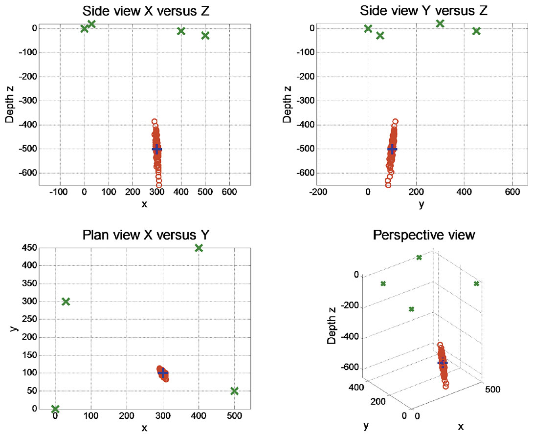
The results for Figure 1 are:
| x0 = 300.00 | y0 = 100.000000.2 | z0 = -500.00 |
| xMn = 299.89 | yMn = 99.856575.2 | zMn = -500.76 |
| xSD = 4.02 | ySD = 6.195285.2 | zSD = 50.07 |
where x0, y0, and z0 are the defined locations, xMn, yMn, and zMn are the mean locations of the 100 trials, and xSD, ySD, and zSD are the standard deviations of the estimated source locations.
The source location is then moved a significant distance to x0 = 2000 m, yielding the results displayed in Figure 2. The spread of the estimated source locations has increased.
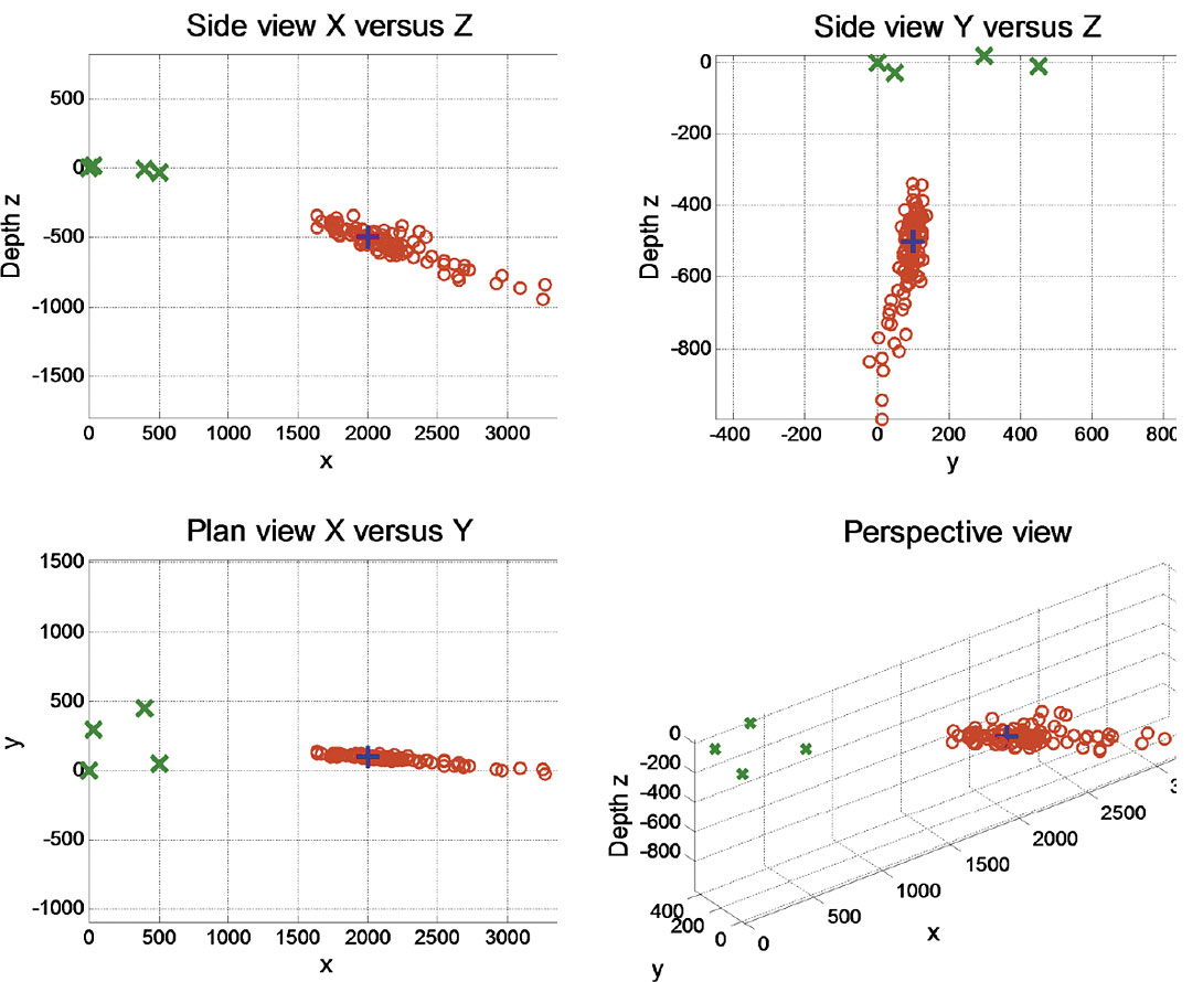
The parameters for Figure 2 follow:
| x0 = 2000.00 | y0 = 100.000000.2 | z0 = -500.00 |
| xMn = 2147.06 | yMn = 89.243578.2 | zMn = -545.99 |
| xSD = 363.21 | ySD = 30.858586.2 | zSD = 128.15 |
The above results are misleading as the actual distribution of the estimated sources is much narrower than the standard deviations would indicate. A more accurate description of the distributed locations would include its shape and direction.
The accuracy of the estimated source location is dependent on its location relative to the receivers. The error of the estimated source depth for a grid of many x and y locations was computed. At each grid point 100 trials were computed, each with different jitter of 1.0 ms. The receiver locations were the same as those in the previous example, and the source depth was maintained at 500 m. An alpha-trim mean was included to remove extreme errors in the estimates of the 100 trials. The trim was 10% off the top and bottom of the sorted estimates. The results of the errors in the vertical components are displayed in Figure 3, which also includes four vertical black lines that represent the location of the four receivers. Some errors in this figure are much larger than shown and are clipped at the maximum values.
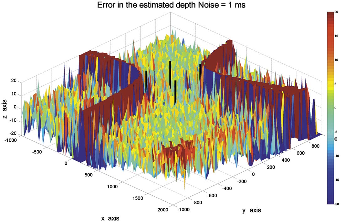
The receiver locations for the data in Figure 3 are:
| x1 = 0 | y1 = 0 | z1 = 0 |
| x2 = 500 | y2 = 50 | z2 = -30 |
| x3 = 30 | y3 = 300 | z3 = 20 |
| x4 = 400 | y4 = 450 | z4 = -10. |
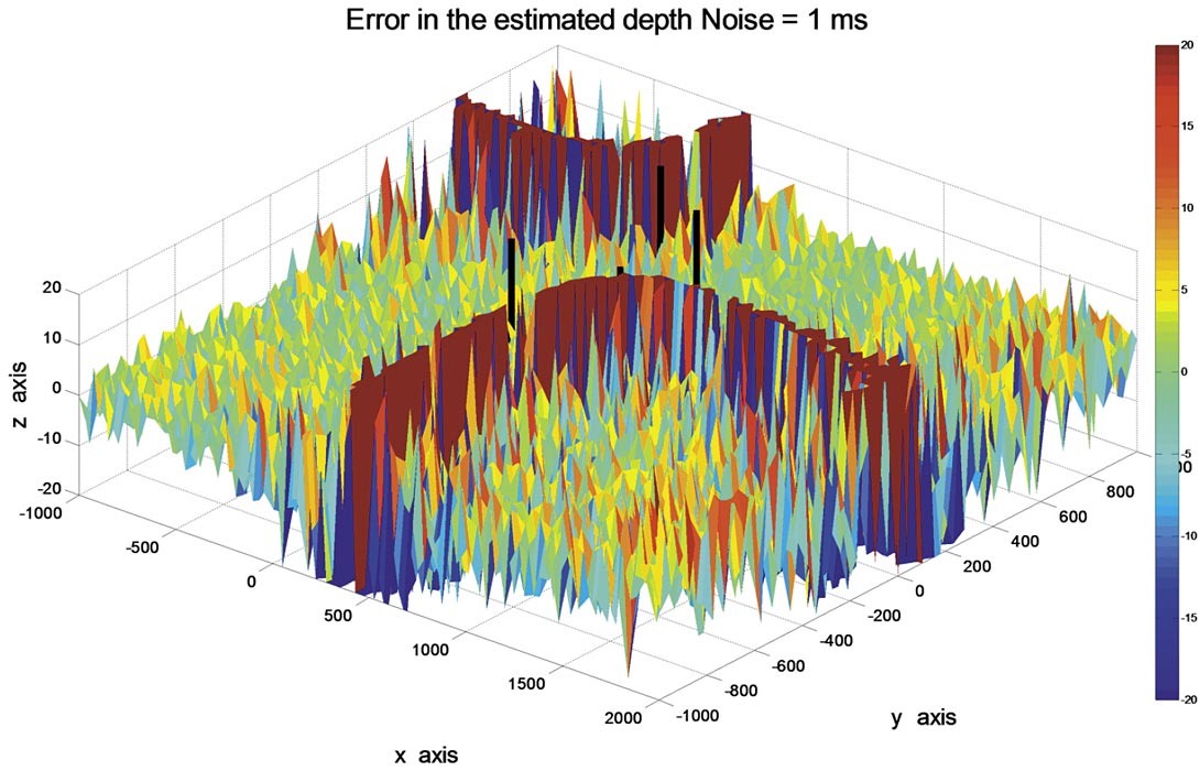
The y location of the third receiver was moved from y3 = 300 m to y3 = 600 m:
| x1 = 0 | y1 = 0 | z1 = 0 |
| x2 = 500 | y2 = 50 | z2 = -30 |
| x3 = 30 | y3 = 600 | z3 = 20 |
| x4 = 400 | y4 = 450 | z4 = -10 |
producing a significant change in the error pattern shown in Figure 4.
Other tests indicate that the areas with poor accuracy appear to be more dependent on the x, and y locations of the receivers, and less dependent on the depth of the receivers.
Sensitivity of four coplanar receivers on a square grid
Data were created for four receivers on a square with a distance of 500 m on each side of the square. One hundred trials were created with Gaussian random jitter, with a standard deviation of 1 ms, added to the receiver times. The results are shown in Figure 5.
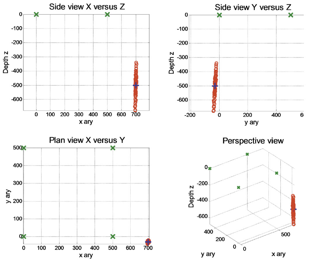
The geometry and results for the data in Figure 5 are:
| x0 = 700.00 | y0 = -30.00 | z0 = -500.00 |
| xMn = 699.55 | yMn = -29.76 | zMn = -501.47 |
| xSD = 2.52 | ySD = 4.55 | zSD = 76.24 |
The source locations were then spread over a large grid and the vertical component of the source SD displayed.
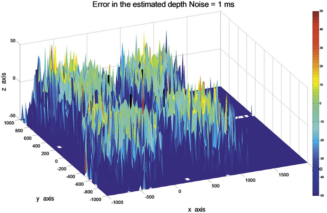
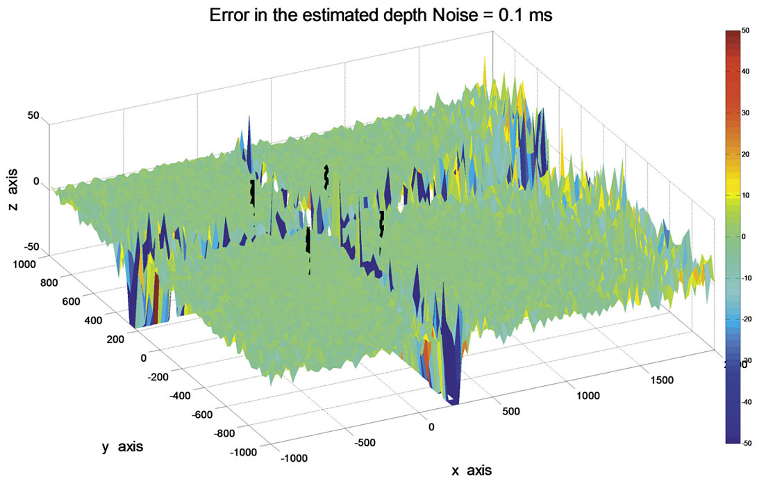
The error in the estimation of the source varies considerably, however, there are areas where the noise is reasonably behaved, but there are also areas where the noise tends to extreme values. In Figure 7, the jitter is reduced to a standard deviation to 0.1 ms, or by a factor of 10. The error in the source estimate is considerably reduced, and valid results cover a much larger area.
Sensitivity of three equally spaced receivers
A simulation of three equally spaced and collinear receivers was conducted. The results are contained in a 2D plane, and if the receivers are in a vertical well, only the depth and radial distance from the well can be computed. A source location was defined and the traveltimes to the three receivers estimated. Using only the receiver geometry and the three receiver clock-times, the source location was estimated. One hundred trials were conducted with jitter added to the receiver clock-times. The results of one set of trials is shown in Figure 8.
Some of the trials failed to produce a location, and the spread was large for a jitter of 1 ms. An alpha-trim (10%) was once again applied. The alpha-trim identified 6 failed computations in 100 tests. The trim size on the remaining samples was 9, and after the 100 estimated depth values we sorted, samples from 10 to 85 were used. The results of the raw data, and with the alpha-trim, are displayed in Figure 8. The Black “+” is the estimated location of the source.
The jitter in Figure 8 (1.0 ms) may be relatively large, so a smaller jitter level of 0.1 ms was added to the receiver clock-times. The distribution of the estimated locations is much smaller in Figure 9, and there were no failed estimates in the raw or alphatrimmed data.
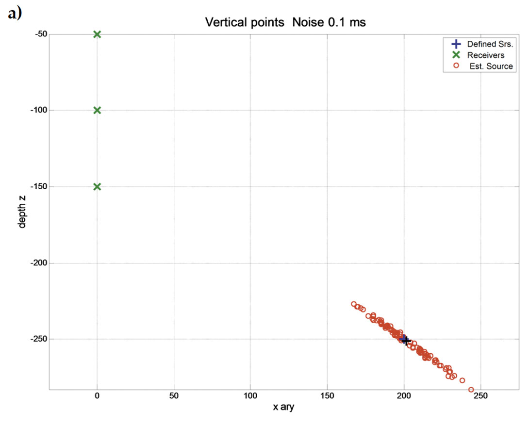
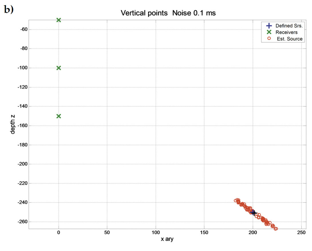
Figure 10 illustrates the results from two sets of receivers, one set at depths of 0, 50, 100 m, and the other set at depths of 180, 200, and 220 m. The source was located at an offset of 200 m and a depth of 150 m. The results display the estimated source locations for 100 tests when a jitter of 0.1 ms was added to the receiver clock-times. The difference in the distribution of the solutions is mainly due to the difference in the receiver interval, i.e., 50 versus 20 m. In addition, the distributions tend to lie on a linear path running from the central receiver to the actual source location. This property, also evident in the previous examples, led to the development of a new method for refining the estimated source location when used with multiple receiver arrays.
Sensitivity of a vertical array of many receivers
The previous examples estimated the sensitivity for each of the analytic solution by using many trials that add jitter to the receiver clock-times. We don’t have that capability in true applications that use many receivers. However we do have the capability to produce many source location estimates by selecting many groups of three equally spaced receivers from the array of receivers then computing the analytic solutions. Consider six equally spaced receivers in a vertical well with a receiver interval h. From these six receivers, we can extract groups of three equally spaced receivers, i.e. 5 groups with interval h, four with interval 2h, three with interval 3h, and two with interval 4h. Each of these fifteen groups will provide an initial estimate of the location and then provide a final estimate of the location (r0, z0) as the mean of the individual components. In addition, the number of initial estimates allows the computation of the standard deviation of the source location.
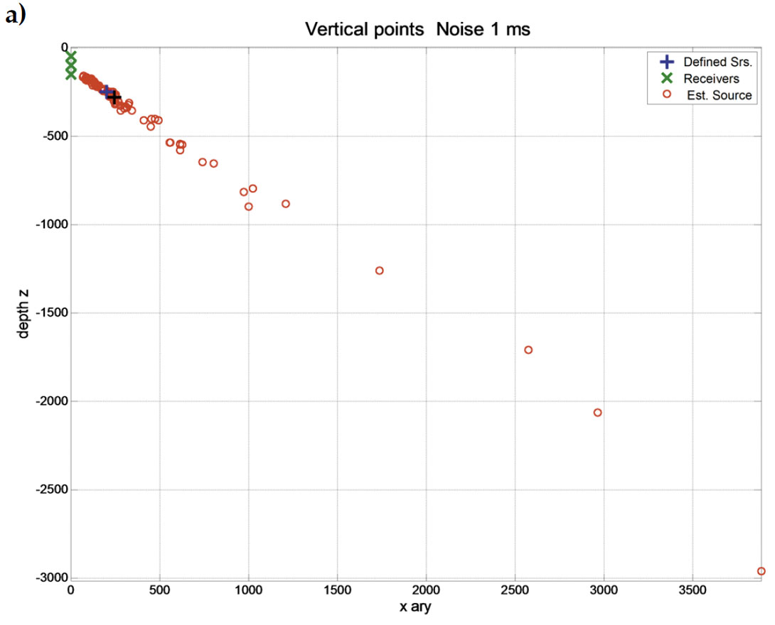
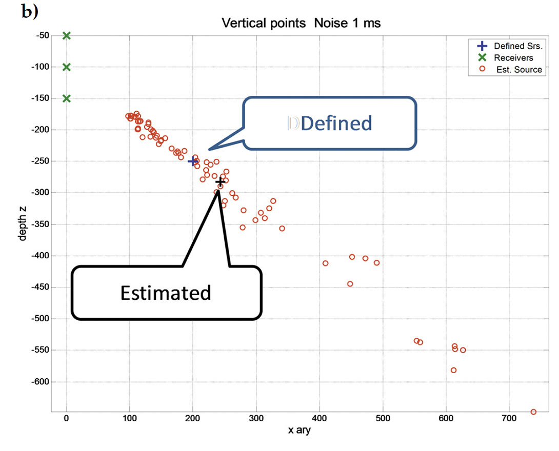
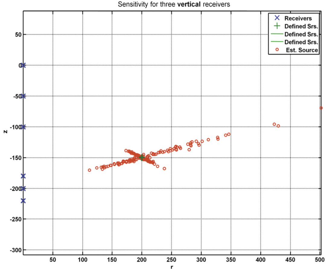
A vertical array of sixteen equally spaced receivers in a vertical well will produces 56 groups of three equally spaced receivers that will be used to compute the sensitivity. The receivers extend from a depth of 100 m with an interval of 50 m to a maximum depth of 850 m. The source is located at an offset of 1000 m and a depth of 400 m. The 56 solutions are shown in Figure 11 where the receiver locations are now in blue. Figure 12a and b show a zoom of Figure 11 with (a) showing a concentration of the estimated solutions close to the actual solution. The mean of the radial and depth components provide a final estimate of the source location, along with the SD. This is referred to as the P (point) solution. Part (b) includes lines from the estimated source location to the corresponding center of the receiver group. The intersection of these vectors produces a new estimate of the source location and is referred to as the V (vector) solution.
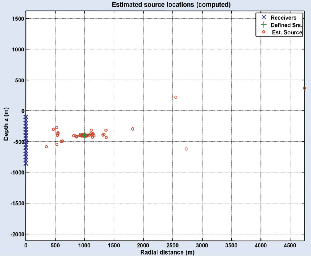
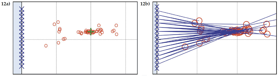
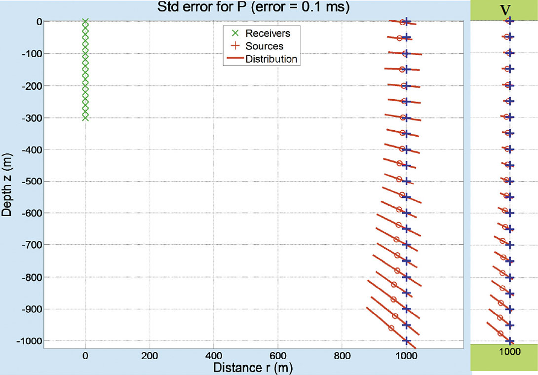
Figure 13 contains a vertical array of sixteen receivers spread from the surface to a depth of 300 m, and a vertical array of twenty one source locations at an offset of 1000 m with depths that range from the surface to 1000 m. Jitter, with a SD of 0.1 ms, was added to the clock-time of each receiver. The estimated source location and the SD are shown for the P and V solutions. In this figure, the V solution is superior. Note the deviation of the estimated location of the sources at the greater depths, and how they tend toward the receivers. This deviation becomes severe for all depths when the jitter is significantly increased to 1.0 ms, as illustrated in Figure 14. While appearing disastrous, note that the discretion of the estimated solutions tend to the true location, and can be corrected with the appropriate numerical techniques. The deviation of the source locations is due to the kurtosis of the distribution of estimates.
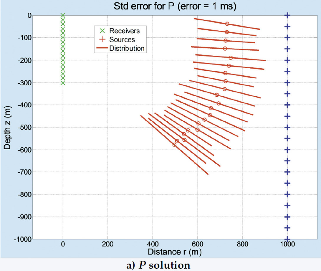
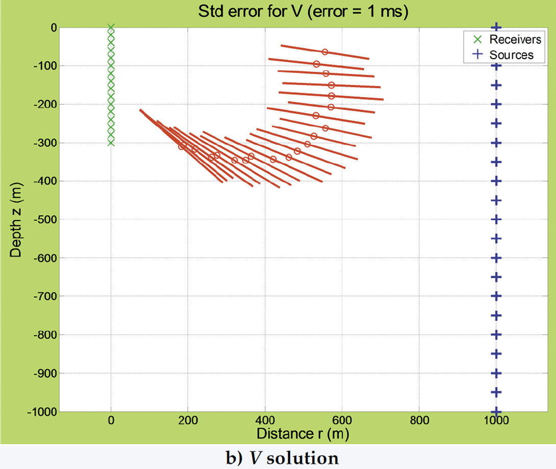
Figures 15 and 16 contain a new configuration of source and receiver locations that illustrate the difference in accuracy when using the first-arrival times of P- and S-waves. A jitter error of 1.0 ms, the same as in Figure 14, is used. Now eight receivers are spread from the surface with increments of 80 m to a maximum depth of 560 m, and the sources located with offset 500 m, and depths that range from the surface to 1000 m. Figure 15 contains the P solution for (a) the P-wave velocities, and (b) the S-wave velocities, and Figure 16 the corresponding V solutions.
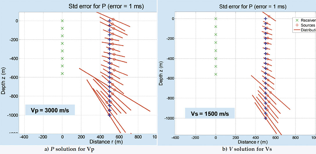
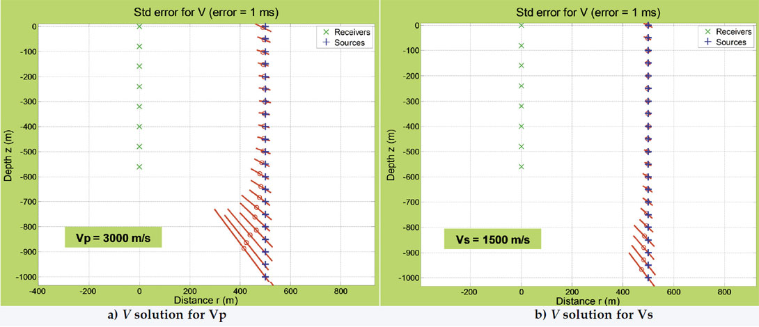
The Improvements in Figures 15 and 16 over Figure 13 are due to:
- a larger spread of the receiver array, even though there are fewer receivers,
- a smaller radial displacement between the source and receiver arrays,
- use of the V rather than the S solution type, and
- a lower velocity for the S-waves.
Comments
The above discussion of the multiple receivers in a vertical well is applicable to a large grid of receivers where multiple groups of four receivers on the corners of a square can be grouped for an analytic solution to estimate the source location and SD of the grid.
It is not possible to pick the exact first-arrival time of the P- and S-waves, but picking the relative first-arrival time between different receivers can be more accurate. An example would be the first peak of the arriving S-wave. Interpolation techniques allow picking a peak with an accuracy greater than the sampling interval, however amplitude noise that is independent from receiver to receiver may distort the location of the desired peak. We feel that a range of jitter from 0.1 to 1.0 ms is reasonable and that the above examples do provide a reasonable expectation of the relative accuracies for the given configurations.
Three-component receivers in a well do allow the azimuthal component of the microseismic event to be estimated. However, greater accuracy would be achieved when using multiple wells. When using only the first-arrival times, less expensive receivers, such as hydrophones, could be deployed in multiple wells that may rival the quality and expense of deploying the multicomponent receivers.
Conclusions
Three analytic methods for computing the location of microseismic hypocenters were presented. Each method only uses the location and first-arrival clock-times of the receivers. The first used the Apollonius solution for four receivers in an arbitrary configuration.
This method fails if the receivers were collinear or coplanar, so two additional methods were presented; four coplanar receivers on a square grid, and three collinear, equally spaced, receivers. The medium was assumed to have a constant velocity, or geometry where RMS type velocities could be used. The sensitivity of the analytic solutions was evaluated by adding jitter to the receiver clock-times.
The analytic solutions were assumed to be part of a larger array of receivers, from which many groups of receivers could be extracted to compute numerous source locations. Jitter was added to the receiver clock-times that enabled an accurate estimate of the location and standard deviation of the source. A vector method was introduced that improved the accuracy of larger receiver arrays.
The accuracy of estimated locations varied with the location of the source relative to the receivers and with the distance from the source to the receivers. The accuracy also varied with the amount of noise added to the receiver clock-times.

Acknowledgements
We wish to thank NSERC and the sponsors of the CREWES consortium for supporting this research.
CREWES: The Consortium for Research in Elastic Wave Exploration Seismology.
We wish to thank NSERC and the sponsors of the CREWES consortium for supporting this research. A special thanks to Kevin Hall for making the graphics printable.
Related Reading


Join the Conversation
Interested in starting, or contributing to a conversation about an article or issue of the RECORDER? Join our CSEG LinkedIn Group.
Share This Article