Seismic waveform shape and character can define facies and reservoir parameters with far greater detail than traditional time and amplitude mapping. Modern techniques using waveform classification make it possible to define and map subtle changes in seismic response and to match them to subsurface information. Waveform classification can also be combined with multi-attribute analysis by concurrently evaluating trends in numerous seismic measurements such as instantaneous attributes, semblance, acoustic impedance and AVO.
This article will focus on some of the various techniques of performing seismic waveform classification including constrained/unconstrained classification and Principal Component Analysis (PCA). A Slave Point carbonate play in Western Canada will be used for illustration purposes.
There are two primary types of classification methods: Unconstrained (Unguided or Unsupervised) and Constrained (Guided or Supervised). An unconstrained classification gives the interpreter insight by showing how a waveform is changing within the survey. Aside from defining an analysis interval, unconstrained classification does not use any a priori information to determine how a seismic trace is classified, and the results are entirely data driven. A neural network quantifies the changes in waveform into discrete segments and the different character types can be displayed as colour variations on a map or profile.
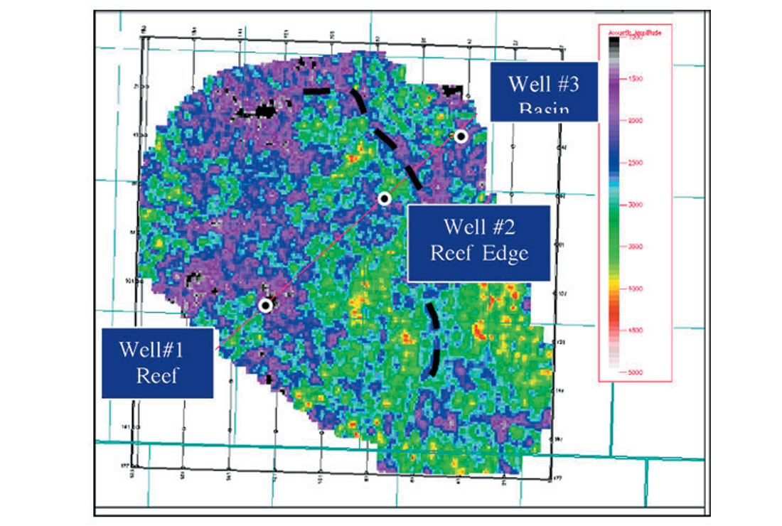
Figure 1 shows an Amplitude Map derived from an interpretation made on the 3D survey. There are three wells: an interior reef well (Well #1) producing gas from dolomitized reef, a limestone reef margin well (Well #2), which is also a gas well but not as porous as (Well #1) and a basin well (Well #3). Although there is an indication of a reef edge, there is no distinctive difference between reef and basin amplitude and the north edge of the reef is very difficult to see.
Unconstrained Classification
An unconstrained waveform classification using three categories, which define the reef, basin and “other” facies, produces the map in Figure 2. Remember that the results are data driven. We have only asked the neural network to divide the waveforms into three groups, without any guidance from the subsurface data about where these character divisions should occur.
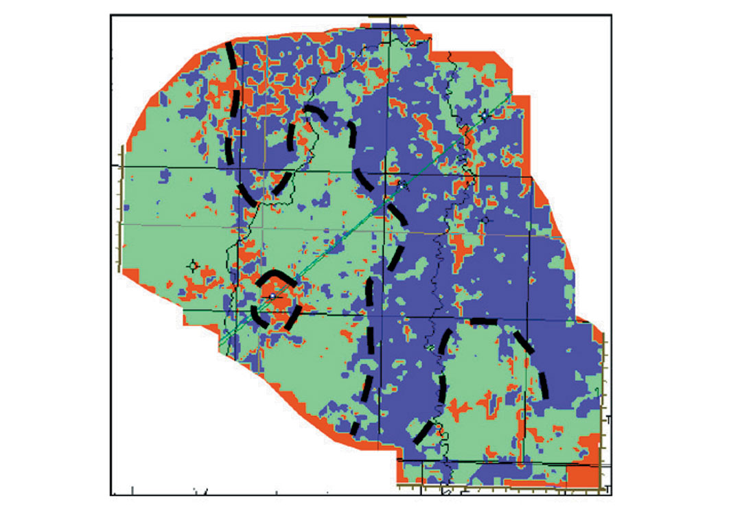
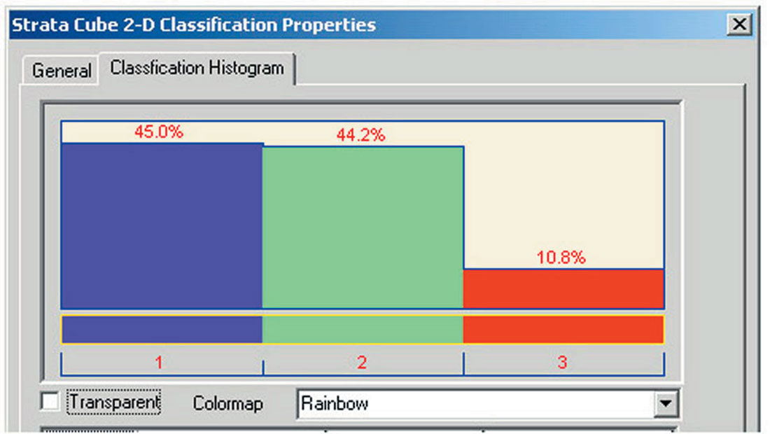
The unconstrained classification result shows a greater distinction between on-reef and off-reef and its general shape is consistent with a basin and reef environment. The histogram (Figure 3) shows that the survey is dominated by traces that fall within one of those two categories. The remaining traces, including the area around the dolomitized reef, are within the “other” category. From well control, we can make the assessment that greens are primarily reef and blues are primarily basin. However, the division between them is not in the correct place because Well #2, porous margin, is in the blue area. There is also a region which appears to be potential reef buildup in the southeast corner of the 3D survey.
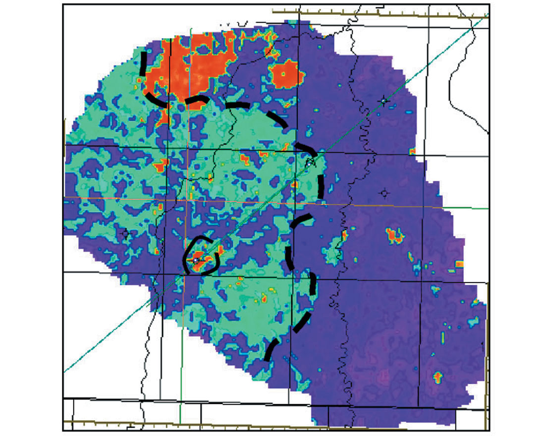
A process known as “Hierarchical Classification” can improve the resolution and further define the geologic changes within the survey. Having separated the traces within the 3D survey into three primary categories, on-reef and off-reef and other, further detail may be achieved by sub-dividing each general classification into a smaller subset, and then taking that subset and subdividing it, and so on. We can say, “Here is the reef, here is the basin, what details can we see within the reef”.
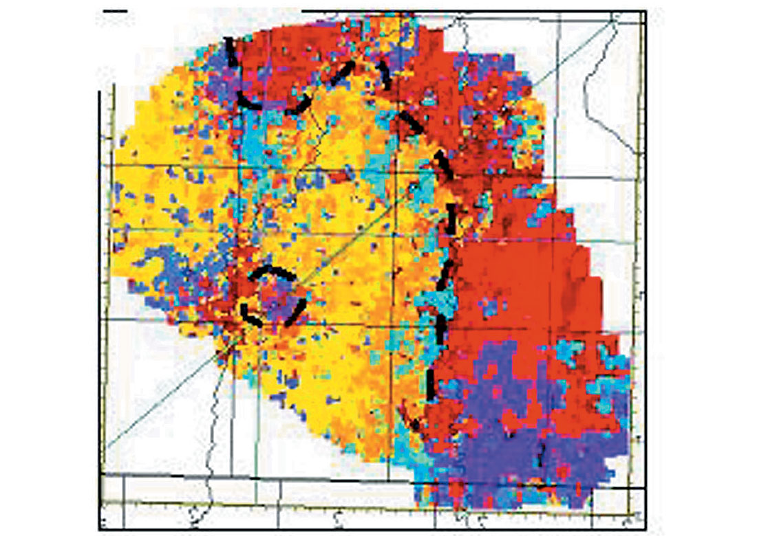
Figure 4 shows the results of hierarchical classification (still unconstrained). Note how the reef margin is much more clearly defined and can be placed in its correct position relative to Well #2. The area around Well #1 has been better defined as an area of possible dolomite development, with waveform character similar to the basinal character. Well #2 is now situated within the reef edge and Well #3 is located in the basin. In addition, the region in the southeast corner of the survey now appears to be basinal and the north edge of the reef is better defined, with the possibility of a reentrant.
As an aside, Figures 5 and 6 illustrate the dramatic result achieved by performing Unconstrained Waveform Classification on a Lower Cretaceous clastic channel.
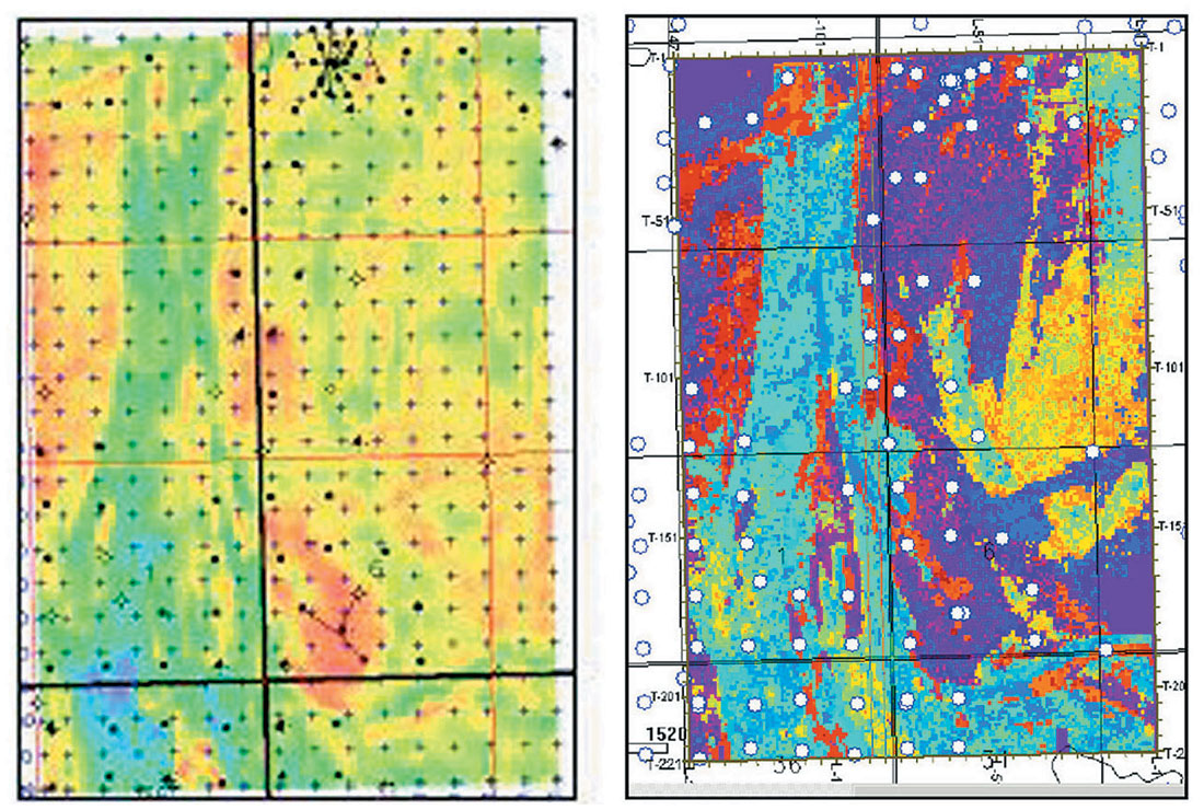
Figure 6. (right) Hierarchical Classification Result
Constrained Classification
Constrained classification uses the known information at specific well locations to classify the seismic data. Instead of saying, “Take all of the traces within the 3D and separate them into 3 (or 8, or 12) categories,” we are saying, “I know what the geology is at the well bore, go and find the matching seismic response.” To achieve this, seismic waveforms that have been extracted from around various well locations (model traces) are compared to each seismic trace (target traces) using a neural network algorithm. The traces are correlated to get a “goodness of fit” and mapped accordingly.
Figure 7 shows the results of a constrained classification using the waveforms extracted around the 3 well locations. It is understandable that the image is different from the unconstrained result as we have told the system what wavelets to use. However, the position of the reef edge and the general shape looks reasonable and this would not be the case unless there was consistency in waveform character.
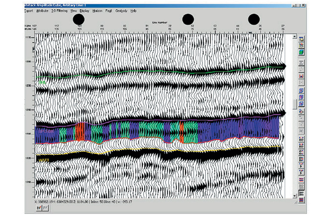
The benefit to constrained classification is that it becomes possible to impart geologic meaning to the cluster analysis. Whereas in unconstrained classification a result is based on how the individual traces in a 3D survey are grouped by their respective similarity (or difference), in constrained classification, a result is based on how well a target trace compares to the model trace. If an interpreter has a good understanding of a seismic signature generated by a specific geologic facies, that waveform can be correlated to the other traces in the 3D. A Waveform Correlation Map can then be derived showing where the target traces have the highest correlation to the known waveform. Projecting the classification results onto a 2D section gives the interpreter insight as to how the seismic data has been categorized (Figure 8).
Multi-Attribute Analysis
Multiple attribute volumes can be derived from a single 3D survey. The most common of these are instantaneous amplitude, phase and frequency, but they may also include acoustic impedance and AVO. Subtle differences within the seismic data are often enhanced or defined by these attributes. A problem arises, however, when an attempt is made to correlate a trend from one volume to another.
One solution to this problem is to use a statistical method called Principal Component Analysis. As with unconstrained and constrained waveform classification, an interval of analysis is used to isolate a seismic signature. “Measurements” such as maximum amplitude, ratio of peak to trough, amplitude slope, etc. are taken over the same interval of each of the attribute volumes.
Principal Component Analysis takes all of the attribute measurements and normalizes them (takes away the units). A data “cloud” is created and an axis system is then fitted to the data which has the direction of greatest variance identified. This vector is the First Principal Component (PCA1). A vector, orthogonal to the first, that describes the second primary dimension for the data cloud is the second principal component (PCA2), then PCA3, etc. Each is orthogonal to the last until all of the data is described. The result is a set of vectors that describes the data set completely. All of the individual, unrelated data measurements have been replaced by vectors.
In this way, Principal Component Analysis reduces the information redundancy within the attribute volumes. It provides a unique solution that is statistically meaningful by ranking those measured attributes that correlate to others. Usually, three or four attributes make up the correlated data set.
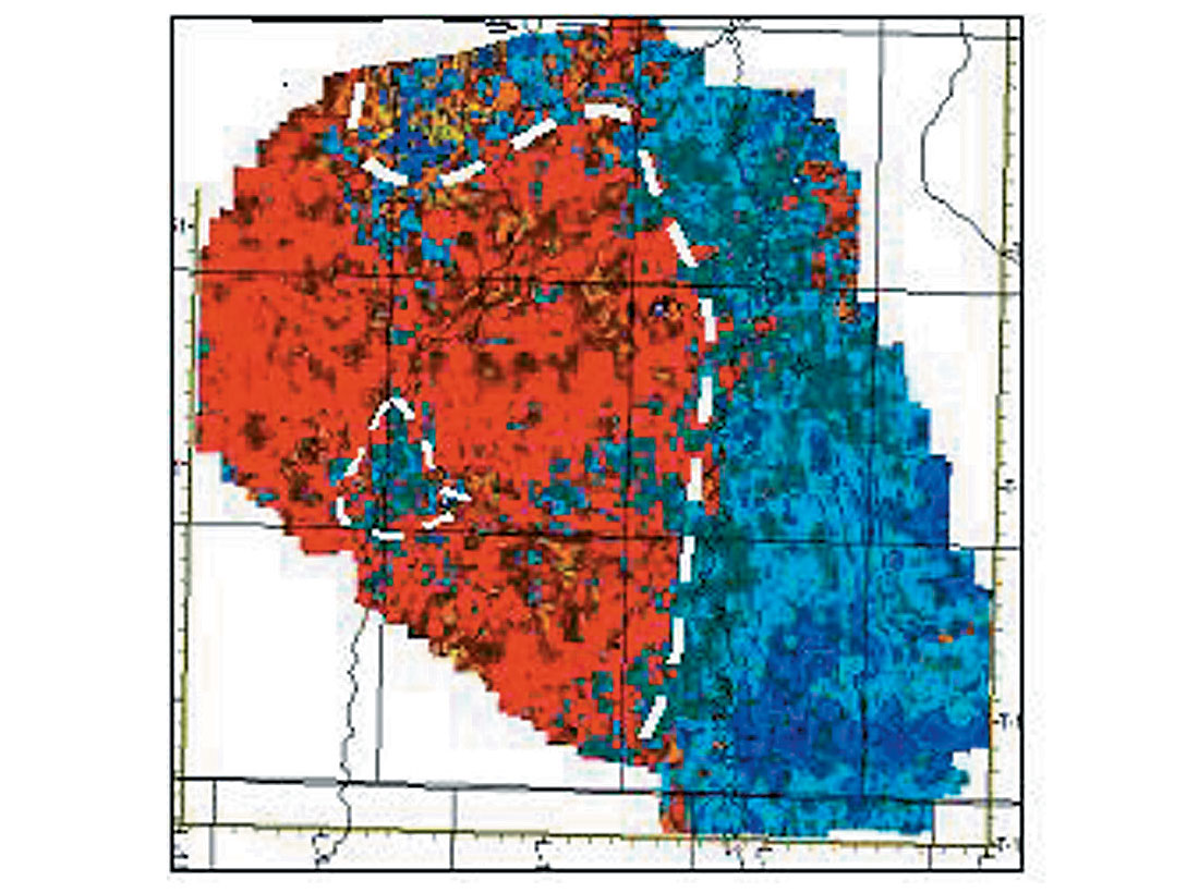
Figure 9 illustrates the result of Principal Component Analysis on our carbonate example. Instantaneous amplitude, phase and frequency are used in conjunction with relative acoustic impedance and post stack amplitude.
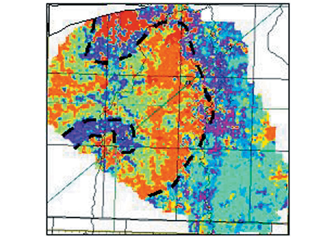
The result is similar to the un-constrained result, except the classes are more distinct, including the area in the southeast corner of the survey. When compared to the hierarchical unconstrained waveform classification (Figure 4), the principal component analysis suggests more strongly that the area of dolomitization extends northward. A basinal reentrant on the north margin is still suggested.
It is this organization of redundant information contained within multiple seismic attributes that allows Principal Component Analysis to excel at waveform classification in areas where well control is limited for a constrained result.
Facies Constrained Classification is a two-stage process. It uses the results of an unconstrained classification, like Principal Component Analysis, by extracting a representative waveform from specific clusters, or facies. It then correlates the waveforms to the seismic data much like a constrained classification. A benefit to Facies Constrained Classification is that boundaries become more apparent and regions of good correlation are easily identified.
In our carbonate example, a waveform is extracted from what is believed to be the on-reef facies, and another is extracted from the basin facies. A waveform correlation map illustrating the correlation between the two facies type is shown in Figure 10. The variations within each of the two colours show the quality of the correlation.
Summary
This Slave Point study is a good example of the different methods we can use to describe and display seismic reflection character. Waveform classification is intuitively obvious and we are simply using the power of computing to assist us, not only with the sort of character mapping that we have been used to, but also to properly identify character differences among many thousands of data points.
Principal component analysis is not intuitive, other than the assumption that we are simply using attribute measurements and their statistical analysis to define seismic character in another domain. It is another way of determining a trend in the data, except it uses data “measurements” (Arithmetic Mean, Slope, Min values, Max values etc) rather than trace samples.
Both the similarity and the differences between the various methods are fascinating because the general results are similar but the fine detail, including possible reservoir extension, is different.

Acknowledgements
The authors would like to thank the staff at Geomodelling Technology Corporation for their continued and timely technical support.


Join the Conversation
Interested in starting, or contributing to a conversation about an article or issue of the RECORDER? Join our CSEG LinkedIn Group.
Share This Article