Seismic Skeletonization: A Useful Tool for Geophysical Data Analysis

1. Introduction

Automated event picking of reflection seismic and georadar data allows an interpreter to analyse coherent events using a variety of statistical tools. The success of such tools in exploration is well-documented (Taner et al., 1979; Robertson and Fisher, 1988; Barnes, 1993; Chen and Sidney, 1997; Marfurt et al., 1998; Schmitt, 1999; Carter and Lines, 2001; Taner, 2001; Barnes 2001; Hart, 2002; Hocker and Fehmers, 2002; Chopra and Marfurt, 2006), although human intervention is required for a complete interpretation of the data.

One pattern recognition technique that has been extensively used in seismic data analysis is called ‘seismic skeletonization’ (Huang et al., 1987; Cheng and Lu, 1989; Le and Nyland, 1990; Lu and Cheng, 1990; Li et al., 1997; Vasudevan and Cook, 1998). Seismic skeletonization is a syntactic pattern recognition method which uses cycles or waveforms as ‘pattern primitives’ that are characterized by features such as amplitude and duration. The number of pattern primitives is dependent on the nature of the data set. Initial efforts by Huang et al. (1987), Cheng and Lu (1989), Le and Nyland (1990) and Lu and Cheng (1990) made no attempt to build a suite of useful attributes for the skeletons for data analysis and interpretation. Li et al. (1997), Cook et al. (1997), Vasudevan and Cook (1998, 2000, 2001), and Eaton and Vasudevan (2004) built an event file (or a catalogue) made up of attributes to seek out information hidden in the data.

Use of the event file for a classical statistical analysis of the reflection data was initially applied to deep crustal reflection seismic data (Vasudevan et al., 1996; Cook et al., 1997; Li et al., 1997, Vasudevan and Cook, 1998). These studies further laid the foundation for the use of the event file to carry out morphological filtering of the reflection seismic data. The scope of the event file is limitless in that as many new attributes derived from pattern primitives or calculated from the data are discovered, new applications may follow.

Eaton and Vasudevan (2004) generalized the skeletonization method of Li et al. (1997) to 2-D grids, thus making it possible to apply the seismic skeletonization method to both seismic and non-seismic 2-D gridded data (Vasudevan et al., 2005). This new approach allows the end-user to define problem specific feature space. It further enables one to scan the data in two orthogonal directions to eliminate or reduce directional bias.

In this note, we describe the current seismic skeletonization algorithm used (Eaton and Vasudevan, 2004) and present results when this algorithm is applied to real data sets. The results allow us to show how the event file (or the event catalogue) can be put to practical use.

2. Methods

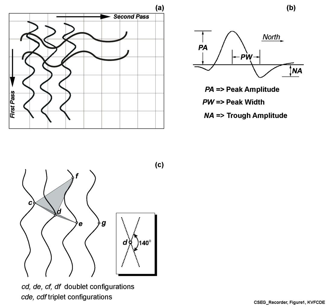
The seismic skeletonization algorithm for a feature space defined by the pattern primitives uses a two-pass approach over a 2-D gridded data. In each pass, events that strike dominantly within a +/- 90° fan perpendicular to the columns of the grid are collected. With two passes, a full 360° azimuthal coverage (including diagonals) is achieved. The following steps are applied:

1. Cycle detection. Cycles are detected by determining local extrema for each column of the data array;
2. Cycle attribute calculation. Each cycle is assigned a suite of attributes, including, but not exclusive to, azimuth, amplitude and pulse-width.
3. Association of contiguous cycles to form event fragments, based on optimization of a cost function;
4. Connection of event fragments to form events. For example, two event fragments are connected at their common cycles to yield a longer event fragment. This process continues until there are no common cycles when the terminated event fragments become events;
5. Event-attribute calculation;
6. Catalogue creation, for subsequent plotting, feature domain filtering and statistical analysis.

We repeat steps 1 to 3 for both the original data matrix as well as its transpose. The event (or catalogue) file resulting from this skeletonization algorithm can be used for data analysis.

2.1. Cycle detection and cycle attributes

Each cycle is an asymmetric waveform consisting of a local maximum (peak) and an adjacent local minimum (trough). The local extrema are identified by scanning through the data in column-sequential fashion. Each peak is paired with the adjacent trough that maximizes the peak-trough amplitude difference (Figure 1). This set of attributes is combined to form a dimensionless “feature” vector:

where λ_MA is a characteristic peak amplitude, λ_NA is a characteristic trough amplitude and λ_PW is a characteristic pulse width, PO is the polarity of the waveform, and T is the transpose of the feature vector. The user-selected parameters λ_MA, λ_NA, and λ_PW are chosen by inspection of representative anomalies extracted from the data. We have found that the algorithm is robust in the sense that it is insensitive to the precise numerical value of these parameters over a range of about one order of magnitude.

2.2. Cycle connection

A search for cycle connections is performed by scanning overlapping three-column ensembles (Figure 1), similar to the binary consistency-checking (Cheng and Lu 1989; Lu and Cheng 1990). For each cycle on the central column in the ensemble, cycle connections are made between either two or three contiguous cycles.

Following Li et al. (1997), we use an optimization procedure to connect cycles based on the minimization of a cost function, Cost. The cost function is a measure of the similarity of adjacent cycles, based on a dimensionless feature vector. Details of the cost function depend on whether the cycle configuration contains two or three cycles. In the case of two cycles, a and b, the connection cost to form a doublet event is represented by a distance measure D(a,b) between the cycles:

where f_a and f_b are the feature vectors associated with cycles a and b, and

where f_i is the i^th component of f. For a triplet configuration, {c, d, e}, the connection cost is represented by

where parameters α₀ and α₁ are user-specified constants that weigh the relative contributions of neighbouring and non-neighbouring cycle correlation (see Li et al., 1997). In the examples given in this paper, we have assigned equal weighting to each of these terms by setting α0 and α1 both equal to 0.5. The term A is given by

where

and

In the special case of 2 or 3 spatial dimensions, the physical representation of the term A in equation (5) is the area of a triangle. This term thus tends toward zero as the three vertices become more collinear. Li et al. (1997) introduced the A term in the calculation of connection cost for a triplet configuration, rather than simply the distance between pairs of points, as a way to honour the local dip information contained within the data. Here, we retain this concept but we have modified the cost function (equation 4) from that used by Li et al. (1997), through the use of A^1/2 rather than A. Our motivation for this modification is to maintain dimensional consistency between the term representing distance (i.e. the term weighted by α₀ and the term representing area (i.e., the term weighted by α₁).

Where multiple connections are possible, the best configuration is selected using the following optimization process. Consider the scenario in Figure 1c, which depicts two possible triplet configurations containing cycle d, cde or cdf, as well as three possible doublet configurations, cd, de and df. The number of allowable configurations is reduced by limiting the search to a prescribed angular aperture of ~140°, and by omitting cycle connections that exceed an empirically determined maximum cost. The selection of an appropriate maximum allowable cost is usually made by testing a small subset of the total area. If any triplet configuration is available, then doublet configurations are excluded. The optimum cycle connection is then selected on the basis of minimizing the connection cost from amongst the allowed set of triplet or doublet configurations. Note that it is possible to connect events of different polarity provided that the connection cost does not exceed the maximum allowed value.

2.3. Event detection and event-attribute calculation

Once cycle connections have been determined, doublet and triplet configurations (event fragments) are joined at common cycles to form events. For example, if cycles c d e and deg (Figure 1c) were connected in the previous step to form discrete triplet configurations, then these two event fragments are connected at the common cycles de to yield a longer event fragment, cdeg. This process of combining event fragments at common cycles is repeated for all cycles to form a complete catalogue of events. Attributes are then computed for each event and stored in the event catalogue. Event attributes include the average value (denoted by the overbar) of the aforementioned cycle attributes, PA, NA, PW, and PO, and as well as the event length, L, average strike direction, q, and norm of residuals, R. For a given event, the length is given by

where dx and dy are the eastward and northward extents of the event. The average event azimuth, θ, is determined by linear regression through the x-y positions defined by cycle peaks. Similarly, R is obtained from the misfit of the linear regression line. Finally, a correction is applied to the pulse-width to account for event obliquity relative to the grid. Based on similar triangles, the corrected pulse width is given by

Since the method is applicable to general 2D gridded data, any pre-processing that would enhance the image of the data may be considered. In the reflection seismic community, coherency filtering of stacked data for interpretation is a common practice. Such filtered data could be input for seismic skeletonization. In the case of aeromagnetic data, edge-enhancement algorithm such as vertical derivative (Keating and Pilkington, 1990) or a 3D analytic signal (Roest et al., 1992) may be applied.

3. Results and Discussion

The 2-D grid skeletonization described in the previous section has been recently applied to reflection seismic data, potential field data and photographic images (Eaton and Vasudevan, 2004; Vasudevan et al., 2005). Event catalogues accrued from the application of the method have been utilized to analyse unique discontinuity features present in each data set. Discontinuity features are characterized by their lengths, orientations, and amplitude strengths and by several attributes derived from the data. As an auxillary step, several more attributes extracted from the data using other means (Neidell and Taner, 1971; Taner et al., 1979; Barnes, 1993; van der Baan and Paul, 2000) could also be added to the event catalogue.

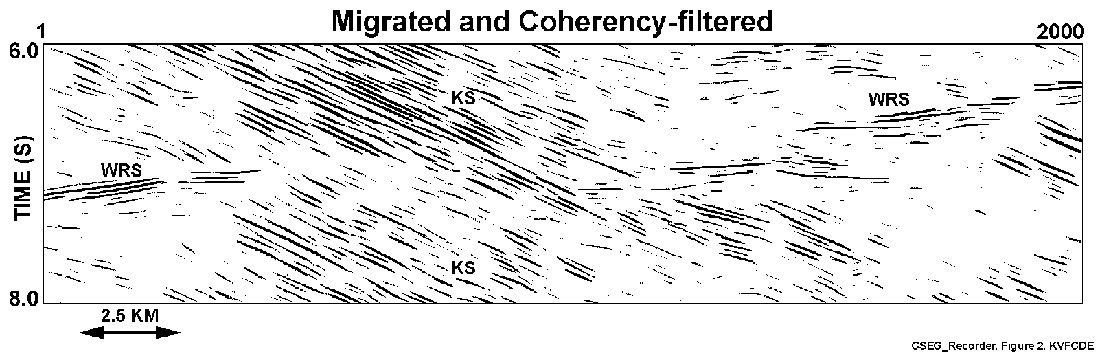
To illustrate the usefulness of the method, we consider two examples, one from deep crustal reflection seismic data and the other from aeromagnetic data. The deep crustal reflection seismic example is from LITHOPROBE PRAISE (Peace River Arch Industry Seismic Experiment) line 12 (Figures 2 through 7), and reveals two strong reflections (Hope and Eaton, 2002; Ross and Eaton, 1997, 2002), one representing the Winagami Reflection Sequence (WRS) and the other east-dipping reflections of Ksituan domain (Ross and Eaton, 2002). The enigmatic WRS extends at least 600 km north-to-south and 200 km east-towest, and is a subject of recent investigation (Welford and Clowes, 2006). We chose a segment of migrated and coherency filtered data of line 12 containing both features. Since they have distinctly different geometry, they are ideal for the seismic skeletonization experiment. The aeromagnetic data example is from the vicinity of the Great Slave Lake shear zone (GSLsz) in northern Canada (Figures 8 through 10). It is from part of the Canadian Shield dominated by linear anomaly trends produced by faults and mafic dikes (Hoffman, 1987; Pilkington and Roest, 1998; Eaton and Vasudevan, 2004). Since this example contains a variety of magnetic anomalies with distinct wavelengths, amplitudes, and directional characteristics, it is an ideal candidate for seismic skeletonization.

Seismic Data Example

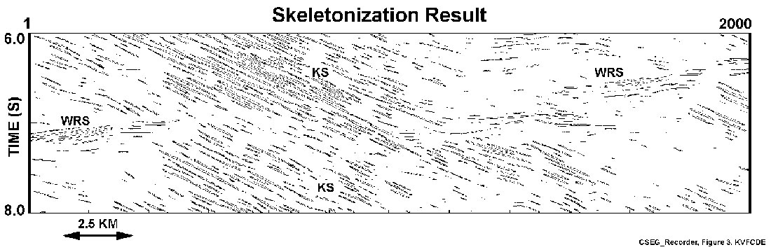
The seismic data example contains 2000 traces in the two-way travel time window of 6.0 – 8.0 seconds. The data were migrated and coherency- filtered (Figure 2). The seismic skeletonization result (Figure 3) displays reflection events of various lengths. The geometry of the WRS feature is made up of sub-horizontal events showing a very gently-west-dipping geometry. In contrast, reflections in the Ksituan domain show strongly-east dipping structure.

The event catalogue resulting from the skeletonization procedure contains information about the events extracted from the data. As a result, attribute-based filtering can be done to understand the statistical behaviour of the data. Here, we consider two examples, one dealing with event-length filtering, and the other directional filtering.

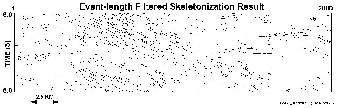
The event map of the seismic section contains variable length events. Although all events may be construed as true events, some of the smaller ones corresponding to event lengths smaller than an event-length of 5 may be associated with noise not removed during the pre-processing phase of skeletonization. To examine the characteristics of longer events, two event-length filtered sections are shown in Figures 4 and 5. For event-length filtering with events less than an event length of 5, the result in Figure 4 shows a better delineation of events than that in Figure 3. Figure 5 reveals an event-filtered length result for an event length less than 16. Figures 4 and 5 suggest the significance of the length-scale of both the WRS and the Ksituan reflections in this part of the data area.

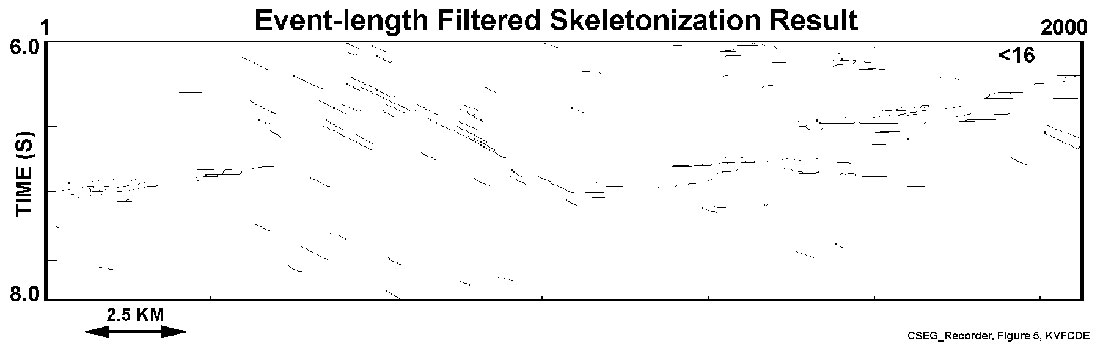
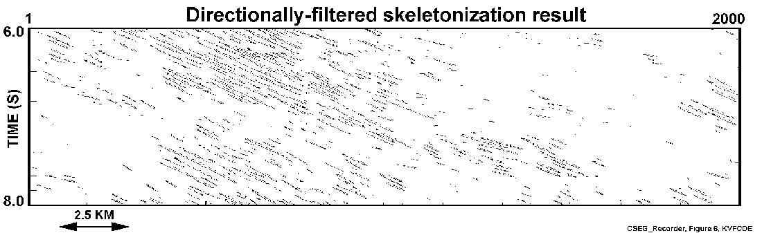
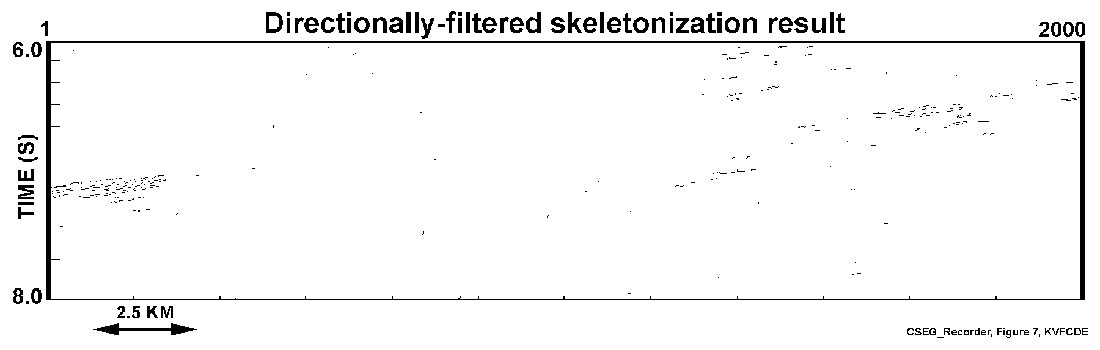
As was pointed out earlier, to separate the two directional features, the WRS feature and the other the shear structure in the Ksituan domain, directional filtering was applied to the event map. Figures 6 and 7 demonstrate the usefulness of the morphological filtering in separating the two event directions that occurred at different geological times. The clean separation of the different dip components by analysis of the skeletonized section may provide an advantage over dip filtering by techniques such as F-K filtering that often add noise during transformation processes.

Potential Field Data Example

The aeromagnetic data were obtained from the Geophysical Data Centre of the Geological Survey of Canada (GSC) in gridded format with IGRF (International Geomagnetic Reference Field) removed. The grid was resampled to 1 km spatial sampling (both x and y) and preprocessed by taking the first vertical derivative. The skeletonization made use of a feature space that includes polarity of the magnetic anomaly. The polarity is normal if the trough of the waveform is closer to magnetic north than the peak, as expected for induced magnetism in the northern hemisphere. Otherwise, the waveform has reverse polarity. The grid of this data set is made up of 350 rows and 222 columns.

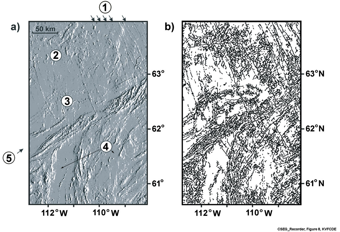
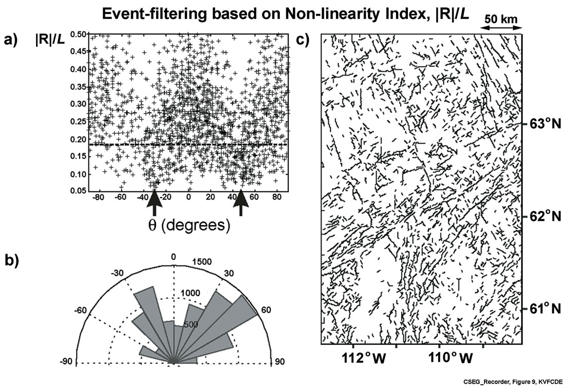
The shaded-relief total-field aeromagnetic map and the event map of the skeletonization process are shown in Figure 8. The skeletonization result reveals all discernible features of the magnetic data, including linear anomalies associated with mafic dikes, cross- cutting fabric elements, and striated anomalies associated with the GSLsz. The input data contain both magnetically quiet and complex anomalous areas and the event map (Figure 8b) reflects this. Since an event catalogue is an automatic end result of skeletonization, statistical analysis and morphological filtering of the skeletonized result could lead to a variety of methods to obtain information from the data. Here, we will be looking at two examples, event-filtering based on information from a so-called nonlinearity index (R / L) (Eaton and Vasudevan, 2004) and strike directions, and directional filtering of the event map.

The skeletonization result in Figure 8 shows a variety of events with different lengths and shapes. Steeply dipping features, such as mafic dikes and the GSLsz, are expected to produce long linear anomalies. The numerous short, non-linear events could mask these features. To address this, we have analyzed the nonlinearity index of all the events as a function of the strike direction (Figure 9a). The results may be filtered by considering events to non-linearity index values within certain limits. In Figure 9b, for example, the distribution of all events for all strike directions with the non-linearity index less than an arbitrarily-chosen value of 0.19 is illustrated in the form of a Rose diagram. This distribution highlights concentrations of events with strike angles in the range of 30° to 60° (GSLsz) and -15° to -30° (Mackenzie dikes). The filtered event map showing events with R / L = 0.19 is represented in Figure 9c and the events present are mostly linear events.

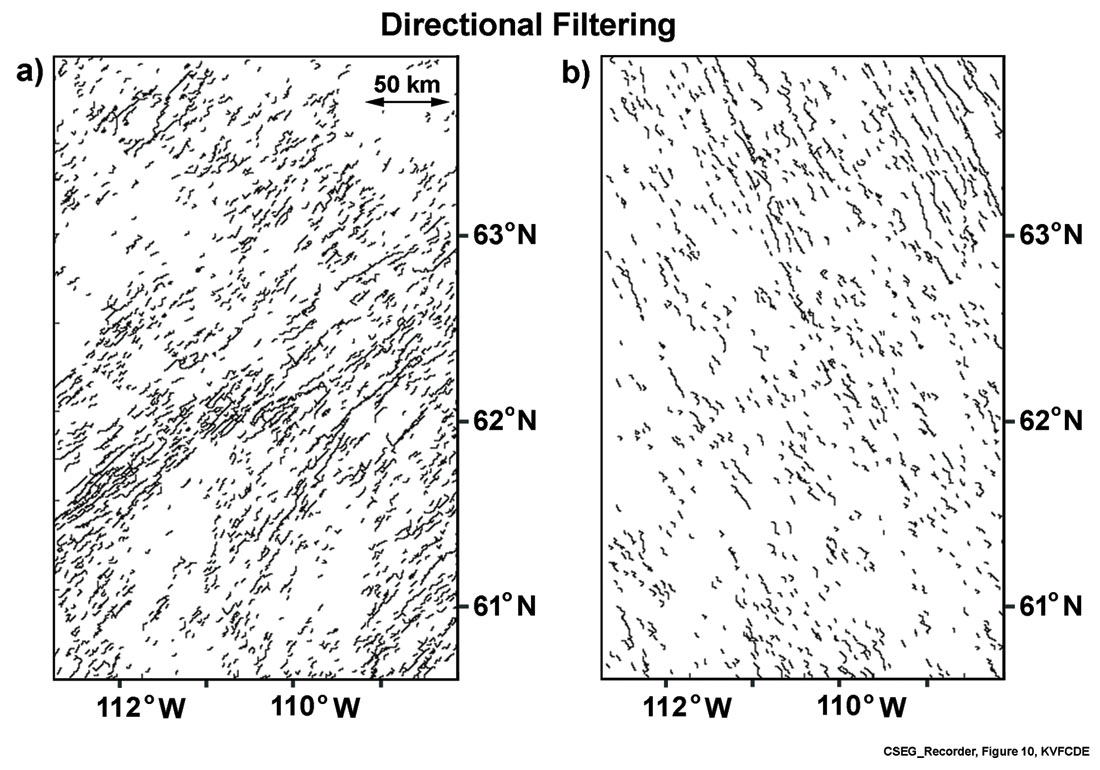
We used the available quantitative distribution of events according to strike directions (Figure 9b) to carry out directional filtering. Results of directional filtering, as shown in Figures 10a and10b, clearly separate out the structural features present in Figure 9c. Events that trend parallel to the GSL shear zone (Figure 10a)and the Mackenzie mafic dikes are clearly evident (Figure 10b).

Conclusion

Seismic skeletonization is a useful tool to generate event maps of different types of data such as the reflection seismic and aeromagnetic data illustrated here. The event catalogue obtained from the procedure can be subjected to statistical analysis to extract a variety of information from the data.

The scope of the analysis and hence, interpretation is determined by the attributes derived from the pattern primitives and location properties, in addition to other attributes externally derived using other signal theoretic methods (e.g. magnetic polarity). Since the seismic skeletons are maps of travel times, future applications such as migration are currently under development.

Acknowledgements

This research is supported by the Natural Sciences and Engineering Research Council of Canada (NSERC). The authors would also like to thank Mark Lane, Qing Li, Charles Hepler, Keith Robley, Peter Tozser, Hugh Geiger, John Varsek and Rolf Maier for discussion and their assistance at the early stages of the seismic skeletonization work. The seismic data were acquired by LITHOPROBE and the aeromagnetic data were provided by the Geological Survey of Canada.