Seismic Physical Modelling at the University of Calgary

Abstract

The University of Calgary Seismic Physical Modelling Facility, in existence since 1985, has been an important tool for seismic exploration research for many years. However, by the standards of the 21st century, it was badly outdated and needed significant improvements. In recent years, we have overhauled and modernized the facility, incorporating such upgrades as a precise six-axes positioning system using linear electric motors and arrays of small ultrasonic source and detector transducers. In addition we have replaced the original electronics with improved circuits for driving source transducers, amplifying detected signals, and signal digitization. Motor control and digital data acquisition are now performed by commercially available circuit boards installed in a modern desktop computer. Once an experiment simulating a seismic survey is set up, it is conducted by the supervisory computer executing customized software within the Windows XP Professional operating system. Automated synchronization of transducer movements and recording of modelled seismic signals from multichannel transmitter and receiver arrays constitute a simple robotics application. Tight integration of the new hardware and software components allows us to efficiently conduct high-fold 2D/3D marine and land seismic surveys with a variety of survey geometries.

Introduction

Scaled-down physical modelling of seismic surveys has been conducted at the University of Calgary for many years. The earliest version of the modelling system, designed and constructed in the mid-1980’s (Cheadle et al., 1985; Lawton et al., 1989), was suitable for generating and receiving ultrasonic pulses in water, and was used to simulate marine-type surveys. Later additions to the equipment enabled reliable contact of transducers to solid surfaces, and made it possible to simulate land surveys. Typically, a scale factor of 104 was used, so that a laboratory experiment over a model with horizontal dimensions of 1000 mm by 800 mm and a vertical dimension of 600 mm scaled up to a real-world seismic survey covering a volume of 10 km by 8 km by 6 km. The transducers produced dominant frequencies in the range of 100 kHz to 500 kHz that scaled down to real-world values of 10 to 50 Hz. Material velocities remained unscaled. Transducers diameters were on the order of about 10 mm, which scaled up to unrealistically large source and geophone footprints of 100 m. Stepper motors driving carriages along aluminum tracks were used to position source and receiver transducers. Rotary motion of the stepper motors was translated into linear motion by sprocket-and-chain mechanisms. Positioning precision and repeatability were poor due to excessive backlash in the mechanisms. Experiments simulating 3D seismic surveys were extremely time-consuming because only one transmitting transducer and one receiving transducer were used. Data precision was limited by available analogue-to-digital (A/D) technology to eight or twelve bits. Software for motion control and data acquisition was originally written in the QuickBasic language and executed on a desktop computer running under MS-DOS. As MS-DOS became obsolete and unsupported, the control and acquisition software was re-written in Java running on a MSWindows PC, but the system was still plagued with hardware accuracy and repeatability issues.

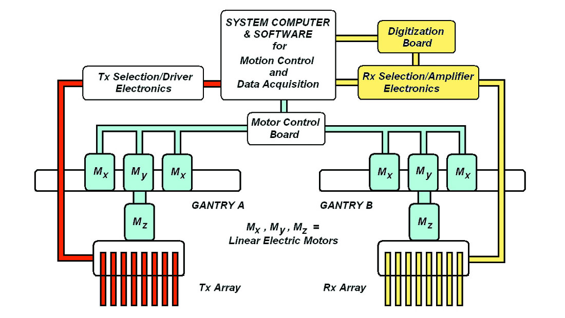
Thus, both the hardware and the software components of the original modelling facility needed significant changes and upgrades. We decided to completely rebuild the facility, replacing obsolete components with modern and improved alternatives. The guiding principle we followed in designing the reconstruction was that the revamped facility must be capable of accurately and efficiently simulating high-resolution 3D seismic surveys in both land and marine environments. In this article, we will describe the system components shown on Figure 1, and briefly document the customized command and control software that has been designed for automated operation of the hardware. We will also present examples from test datasets acquired with the upgraded physical modeling facility.

The positioning system

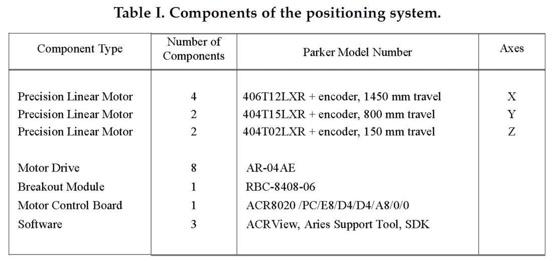
The new positioning system employs modern linear electric motors with sophisticated motion controllers from Parker Motion Corporation (Bland et al., 2006; Wong et al., 2007). Table I lists the components used in the positioning system. The motors require 60 Hz-120 VAC power and can draw up to 35 A at maximum load. They are capable of lifting more than 100 kg each. This load-bearing capacity is not required for our application, since we use them to move and position transmitting and receiving transducers weighing much less than 1 kg. More germane to our needs is the fact that each motor/encoder/drive combination is capable of moving and positioning with a precision and repeatability of less than 0.1 mm. The motors are capable of accelerations and velocities of more than 104 mm/s² and 10⁴ mm/s, respectively. For safe, human-unattended operation in the modeling facility, we limit these values to no more than 50 mm/s² and 50 mm/s.

The eight linear motors with position encoders and motor drives are configured in a two-gantry orthogonal motion system. Each gantry has 4 motors. Two of these motors work together to move the gantry in the X direction. The two remaining motors are mounted on the gantry so as to move an equipment carriage in the Y and Z directions. Transmitting and receiving transducers that generate and detect ultrasonic seismic pulses can be mounted interchangeably on the two gantry carriages and be moved precisely and independently in all directions.

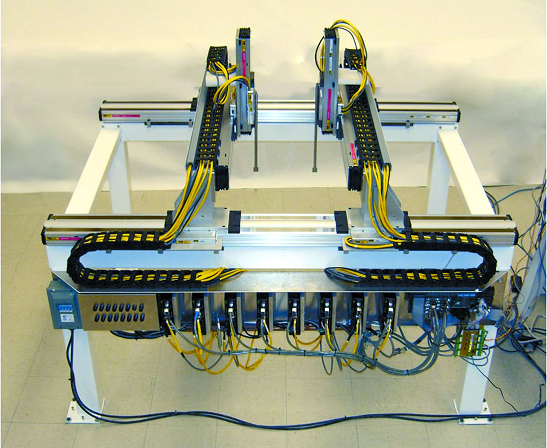
Figure 2 shows the two gantries, AC power switches and fuses, eight motor drives, and motor controller mounted on a steel frame. The frame has dimensions of 1800 mm long by 1200 mm wide by 900 mm high, and scaled-down physical models with dimensions smaller than these can be placed within the frame beneath the gantries. After installation on the frame, the maximum ranges of motion for the X, Y, and Z motors are 1100 mm, 800 mm, and 150 mm, respectively. The standard scale factor is 10⁴, so these dimensions represent a realworld volume of 11.0 km by 8.0 km by 1.5 km. On the figure, the left gantry is designated Gantry A, and the right gantry is designated Gantry B. The coordinate system is set up so that positive X is to the right, positive Y is into the page, and positive Z is down. The eight motors on the two gantries are controlled by computer commands issued to an AR-8020 motor controller board installed in a desktop PC running the Windows XP Professional operating system.

Piezoelectric transducers and transducer arrays

Piezoelectric transducers may be used interchangeably as ultrasonic transmitters or receivers in experiments simulating seismic surveys on land or sea. When a piezoelectric material is subjected to a time-varying high voltage signal, it responds by generating mechanical vibrations that follow the voltage. Alternatively, if the piezoelectric material is mechanically deformed by vibrations, it produces a low-voltage signal. The transfer functions between voltages and deformations are highly stable, so that stacking of signals produced by repeated identical transmitter high voltages is possible. The most common piezoelectric material used in commercially available transducers is a ceramic solid known as lead zirconate titanate (PZT).

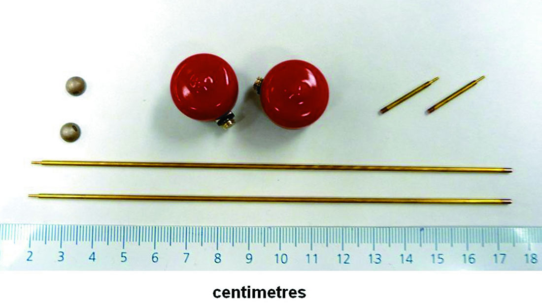
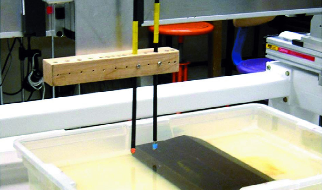
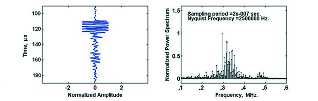
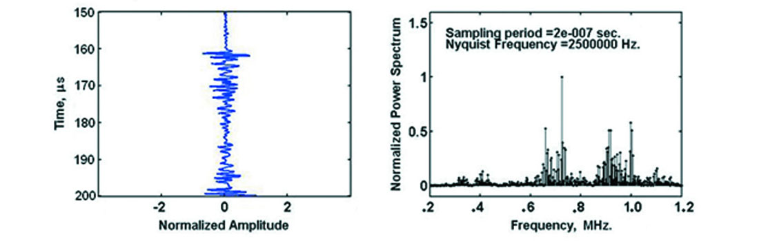
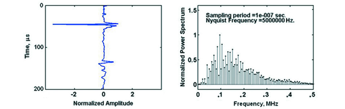
Piezoelectric transducers come in different shapes and sizes. Figure 3 shows examples of three types: hemispheres, cylinders, and piezopins. The hemispheres have diameters of 6 mm. The larger cylinders are called V103 transducers and have active elements with diameters of 12.7 mm. The piezopins are very small cylindrical piezoelectric elements (approximately 1 mm diameter by .5 mm long) bonded to the tips of thin metal tubes (about 1.6 mm diameter by 150 mm long). Each type has particular advantages and disadvantages for scale modelling, and we may choose a specific type to use in a particular experiment. For a given applied high-voltage pulse, the larger cylindrical and hemispheric shapes produce stronger vibrations with lower dominant frequencies (on the order of 100 to 400 kHz). Figure 4 shows two hemispheric transducers bonded to the bottom tips of long rods and mounted on Gantry A. Piezopins tend to produce higher dominant frequencies (about 600 kHz to 1.2 MHz), so their signals can resolve finer geometrical details. Figure 5 is a photograph of an array piezopins mounted on Gantry A. Figures 6 to 9 show examples of seismic traces and their power spectra for various combinations of source and receiver transducers on water and solid surfaces.

With a scale factor of 10⁴, the 1-mm diameters of the piezopins mimic real-world source/receiver footprints of 10 m. This is a great improvement over the larger cylindrical V103 transducers, whose diameters of 12.7 mm scale up to unrealistically large realworld footprints of 127 m. However, the larger transducers produce stronger signal levels that may be needed when large transmitter-receiver offsets are involved. Because of their small size, piezopins are well-suited for constructing arrays of multiple transducers. In any model experiment, moving transducers to their desired positions is the most time-intensive operation. By employing multichannel receiver and transmitter arrays, we can decrease the number of transducer moves significantly, and so increase the efficiency of conducting experiments that simulate high-resolution 3D surveys. To achieve added flexibility for setting up survey geometries, the transducer array was designed so it can be mounted horizontally on the gantries in orthogonal directions. The piezopins are spaced 10 mm apart, and each one of them can be connected either as a receiver (Rx) or a transmitter (Tx). Each piezopin is spring-loaded vertically, so that by moving the Z motors down, the active tips of the array can be coupled consistently to a solid surface for modelling land-type surveys (the solid surface should be covered by a very thin layer of silicon grease or hydraulic fluid to improve coupling).

Transmitter and receiver electronics

A transmitting transducer is driven by a circuit that generates a high-voltage square wave with a very high slew rate on the falling edge (the voltage falls from 325 volts to zero in less than a microsecond). The transducer responds to the sharp decrease in voltage, and reacts to the derivative of the square wave (which is a series of sharp pulses) by producing ultrasonic seismic pulses. The dominant frequency of each seismic pulse is strongly dependent on the physical shape and dimensions of the particular piezoelectric transducer, as well as on the acoustic impedance of the material to which it is coupled.

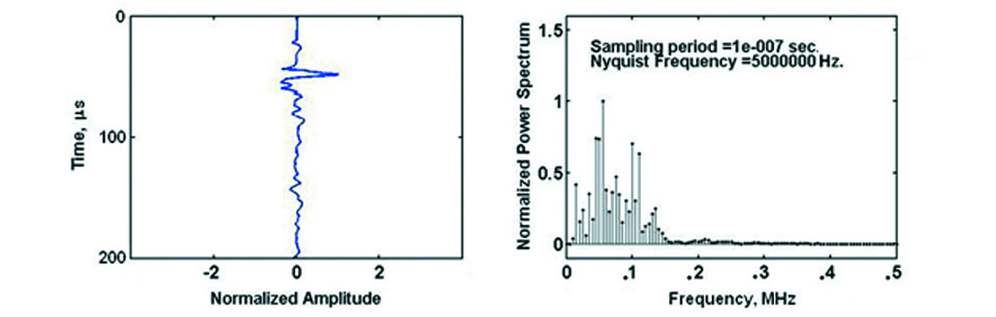
Areceiving transducer senses ultrasonic vibrations and produces a voltage signal proportional to the vibration pressure. Preamplifiers based on high-frequency operational amplifier integrated circuits are used to boost the voltages produced by receiving transducers. Typically, the preamplifiers are built with gains of about 1000 (60 dB), high-cut corner frequencies at 2 MHz, and roll-offs of 12 dB/per octave for anti-aliasing filtering. The amplified signals are routed to a Compuscope CS-1450 A/D board installed in a PCI slot on the system computer. The board has two input channels, and it can digitize input signals with 14- bit precision at rates as fast as 25 megasamples per second. Our standard sampling interval for digitization is 0.1 microseconds, so the high-cut corner is well below the Nyquist frequency.

Multiplexing circuits are needed to select and activate individual transmitting and receiving transducers in the multichannel arrays. We have designed and built customized selection circuits controlled by eight open collector outputs on the Parker-Hannifin RBC breakout module listed on Table I. The breakout module is tied to the ACR-8020 motor controller board mounted in a PCI slot on the system computer. The open collector outputs can be turned on or off by software commands issued by the computer.

Master program for motion control and data acquisition

Positioning of transducers and selection of Tx/Rx transducers are enabled by software commands issued to the ACR-8020 motor controller board. Digitization and recording of ultrasonic seismic data are controlled by software commands issued to the CS-1450 A/D board. Both boards are designed by their respective manufacturers to be installed in PCI slots and come with software development kits (SDKs) for the Microsoft Visual Studio Integrated Development Environment. We used these SDKs to develop a customized master program using C and C++. The master program defines and synchronizes essential functions needed for automatic seismic surveying: motion and positioning control, selection and activation of transmitting and receiving transducers, digitization of seismic traces, and output of seismic data to SEG-Y files with acquisition and geometry information in the trace headers. The master program accepts minimum, maximum, and increment values for the X, Y, and Z coordinates, and proceeds to automatically acquire 2D or 3D ultrasonic seismic data over the defined survey area. Suitable checks are included in the software to prevent collisions between gantries during automatic movements.

Examples of model test data

Measurements on water surface

Figure 10 is a schematic diagram of a physical model simulating a marine-type survey using an array of eight piezopin transmitters and two piezopin receivers. The horizontal dimension is about 400 mm. The depths of the water to the top of the plexiglass body, top of the phenolic body, bottom of container are 112 mm, 82 mm, and 138 mm, respectively. The array was moved from left to right in 2 mm increments over the centres of the targets, covering a total distance of 300 mm in the Y-direction.

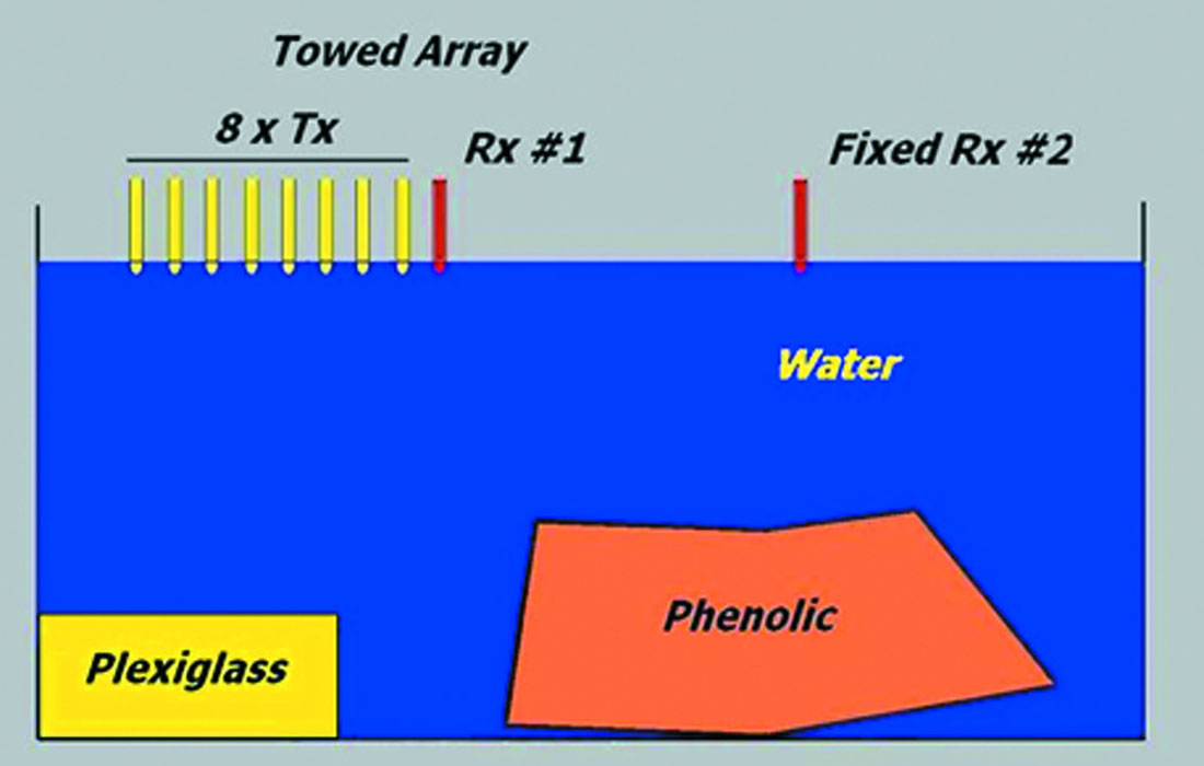
Common offset gathers were recorded with receiver Rx #1 which is part of the moving linear array. Source-receiver offsets in the array range from 10 mm to 80 mm in 10 mm steps. As well, common receiver gathers were collected with receiver Rx #2, located at a fixed offset of 20 mm from the line.

Figure 11 shows a common offset gather with Tx-Rx offset of 40 mm as normalized and AGC displays. The reflection from the top of the plexiglass body appears on the left edge of the displays at a time of about 155 μs. The reflection from the bottom of the container holding the water occurs at about 180 μs. The reflection from the top of the phenolic body arrives at about 100 to 110 μs. When AGC is applied, we can clearly see the weak diffraction patterns originating from the corners of the two solid bodies.

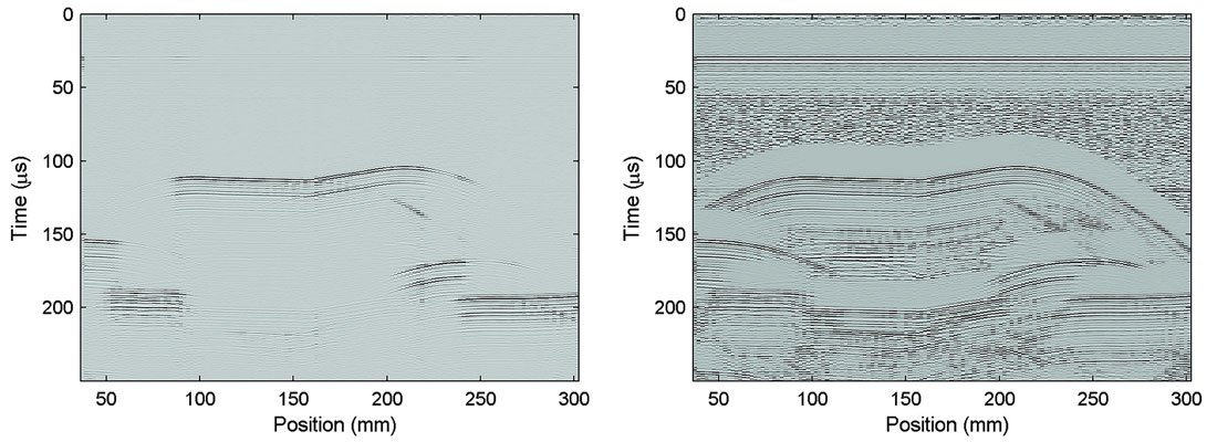
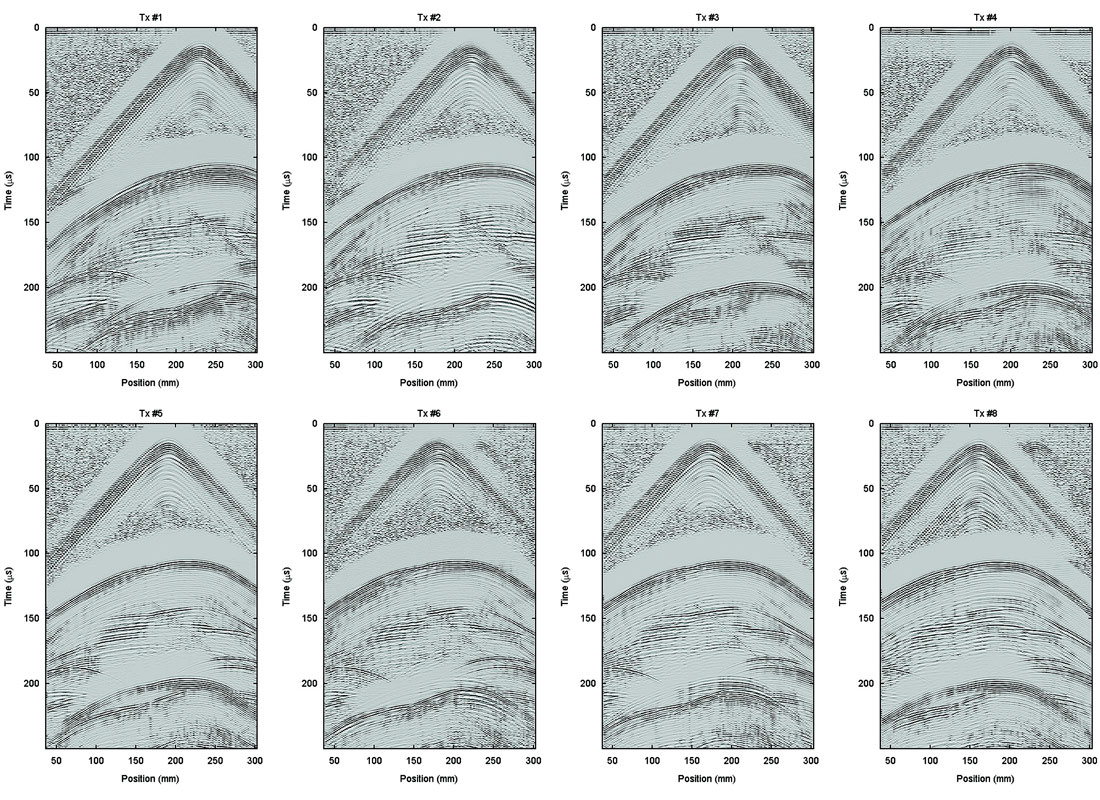
Figure 12 shows eight different common receiver gathers associated with the fixed receiver Rx #2 and the eight different transmitters shown on the Figure 10 schematic. Detailed examination of the common receiver gathers on Figure 12 indicates that, while the waveforms of the primary reflections are reasonably consistent from one transmitter to another, the character of multiples and events coming from below the top of the phenolic body vary noticeably from source to source. The reason for this variability may be differences in the piezoelectric characteristics from transducer to transducer, coupled with subtle differences in the mechanical mounting of the transducers. The waveform variability in the gathers may be decreased by deconvolution. However, it is likely that a procedure for selecting transducers with well-matched responses will be required for better results.

Measurements on solid surface

Measurements on solid surfaces, required for simulating land reflection surveys, are more difficult to make. Consistent and firm contact between transducers and the solid surface must be ensured. We have done this with the array of piezopins by loading each piezopin transducer with a spring, as is shown on Figure 5. A thin layer of grease or oil on the solid surface greatly improves the coupling to transducers. Physical modelling of surveys on solid surfaces is complicated by the fact that strong surface waves are generated that obscure reflections.

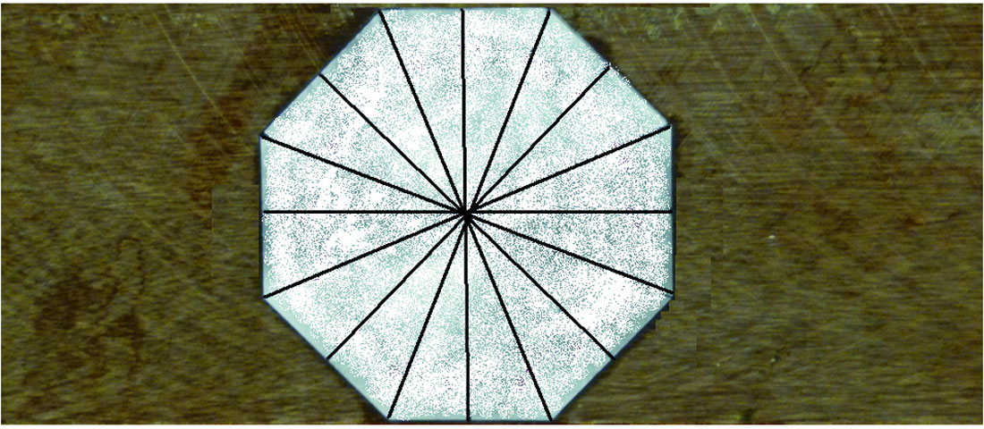
A set of test measurements was made on the phenolic body shown on Figure 13. Phenolic is a composite material consisting of layers of woven cloth bonded by resin. The result is an anisotropic solid with density of 1360 kg/m³, low velocities (about 2900 m/s) across the laminations, and high velocities (3300 to 3600 m/s) along the laminations (Brown et al., 1991; Cheadle et al., 1991). The laminations within the phenolic can be clearly seen on Figure 13. A pair of Tx and Rx transducers separated by 80 mm was placed on the straight lines of the octagon pattern, systematically covering the directions between perpendicular to the layering (i.e., 0 , 180, and 360 degrees) and parallel to the layering (90 and 270 degrees). Figure 14 shows the seismograms obtained as the propagation angle changed; the anisotropy of the phenolic is clearly evident in the arrival times of the P-wave and the surface wave. As expected, the longer arrival times are in the direction perpendicular to the laminations. The P-wave velocities determined from the first arrival times are between 2670 m/s and 3540 m/sec. The surface-wave velocities calculated from the second arrival times are between 1360 m/s and 1540 m/s. These latter values are consistent with anisotropic shear wave velocities (1500 to 1660 m/s) reported for phenolic by Cheadle et al. (1991).

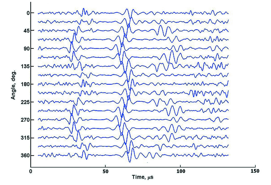
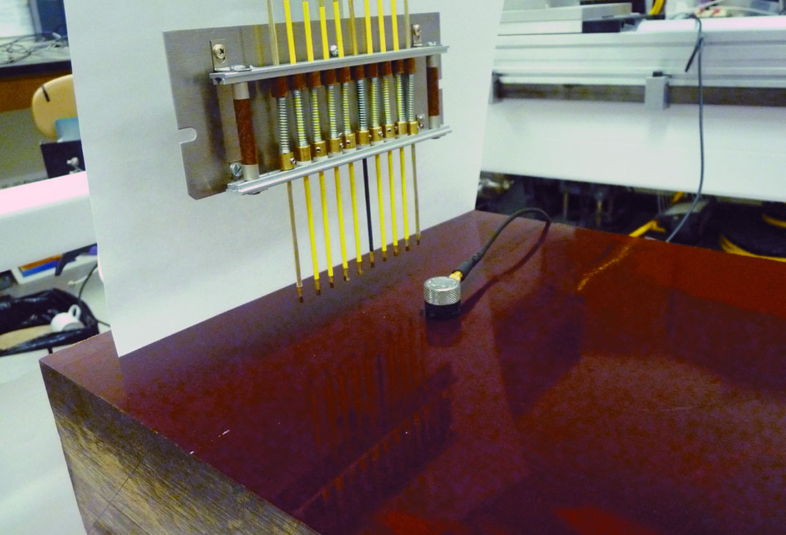
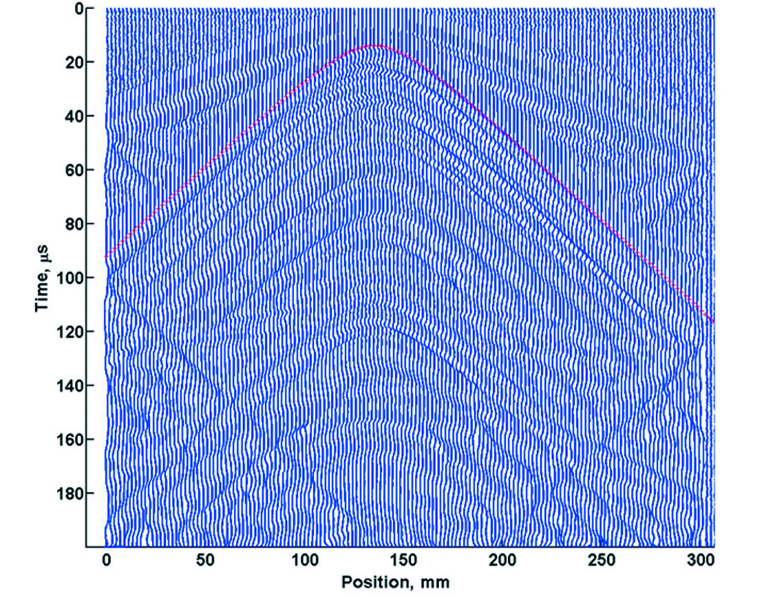
Figure 15 shows an array of piezopin receivers and a V103 transmitting transducer on the top surface of a phenolic block with horizontal dimensions of 300 mm by 300 mm. The phenolic is 105 mm thick and rests on a second PVC block 40 mm thick. The PVC body is supported in such a way that the bottom surface is in air. Phenolic has a P-wave velocity of 2900 in the vertical direction, and a density of 1380 kg/m³ , while PVC has a P-wave velocity of 2350 m/s and a density of 1300 kg/m³ (Cooper et al., 2007). This model has two reflecting boundaries at depths of 105 mm and 145 mm, with reflection coefficients of -0.14 and -1.00, respectively. A common-source gather was recorded by moving the receiver array in 2 mm intervals in the Y-direction (parallel to the receiver array) in an attempt to observe reflections in a land–type simulation. The V103 source transducer was offset about 20 mm from the receiver line. Figure 16 shows the resulting unprocessed common-source gather in an AGC display. The phenolic P-wave velocity estimated from the flanks of first arrival hyperbola is about 3450 m/s, consistent with values reported by Cheadle et al. (1991) for P-waves travelling along the laminations of the phenolic block. The surface-wave velocity estimated from the flanks of the surface-wave hyperbola is about 1500 m/s, again consistent with shear wave values reported by Cheadle et al. (1991).

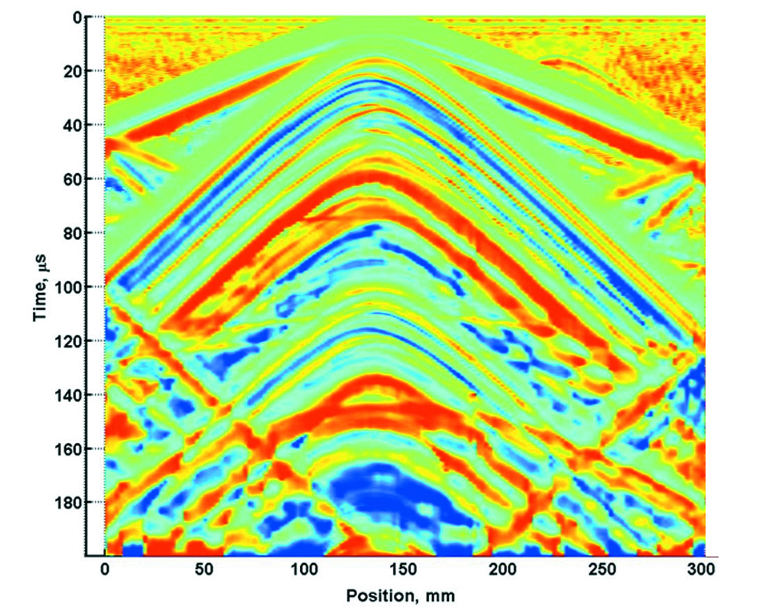
The raw gather is dominated by source–generated surface waves and their multiples that overwhelm any P-wave reflections. The surface wave multiples are due to echoes of the source pulses up and down the lengths of the piezopins. The surface waves and their multiples must be eliminated in order to see the reflections more clearly. Figure 17 indicates that most of the surface waves and their multiples show a characteristic hyperbolic moveout described by the familiar equation

t² = t_o² + (y-y₀) ²/v².

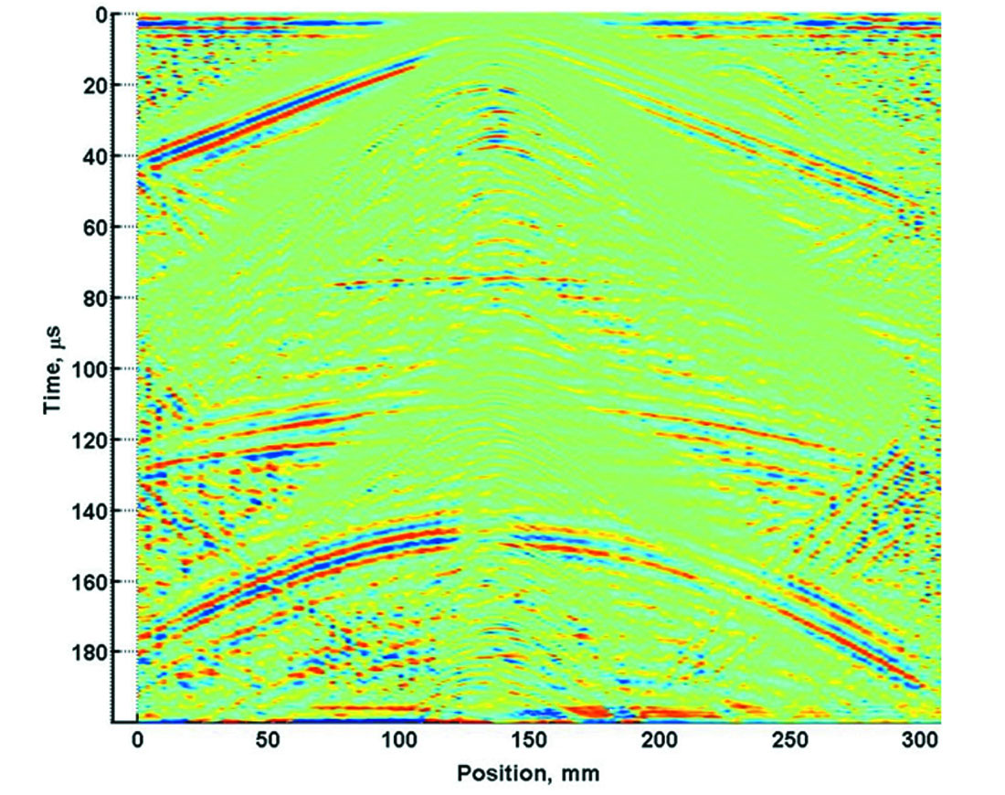
The red line shows a fit to the primary surface wave arrivals using t_o = 14 µs, y₀ = 134 mm, and ν = 1480 m/s. After timeshifting the traces on the gather to flatten the hyperbolae, we used wavenumber filtering to mute the flattened events, and then reversed the time shifts.

The result is displayed on Figure 18. Reflection events with apexes near 74 μs and 108 µs can now be seen. The first time corresponds to the two-way vertical path to the 105 mm depth phenolic/PVC boundary with a velocity of about 2800 m/s. This value is close to the P-wave velocity perpendicular to the laminations of the phenolic body (Cheadle et al., 1991). The second time of 108 µs includes the interval two-way time through the PVC with a velocity of about 2350 m/s. The low-velocity, highamplitude reflection below 140 µs is a surface-wave reflection from an edge of the phenolic block parallel to and about 100 mm offset from the survey line.

Summary and discussion

Just as seismic acquisition technology has evolved and improved tremendously over the past three decades, so the U of C Seismic Modelling Facility has grown in its sophistication and capability. We have described the modernized hardware and electronic features of the facility in its current state. We also have given the broad outlines of the software designed and written by CREWES personnel to control and synchronize the workings of the hardware.

Optimization of the system is on-going, and we continue to identify areas where improvements need to be made. For some experiments, transducers more responsive than piezopins will be required. We must explore ways of attenuating the strong surface waves observed when modelling on solid surfaces before digitizing the signals. We also need to investigate improvements to receiver amplifier and transmitter driver circuits and the use of frequency sweeps and pseudorandom pilots for driving the transmitters. In addition, we need to be able to simulate multicomponent seismic surveys.

At present, the modelling facility can acquire and store up to 2000 traces per hour, with each trace representing a vertical stack of 100 individual waveforms. For simulating high-resolution 3D surveys, we expect to collect datasets on the order of 10⁵ traces or more. To decrease the time required to collect such large datasets, we want to increase the acquisition rate to 10,000 traces per hour. For this to happen, expansion of the transmitter and receiver arrays to 16 or 32 elements is desirable. We will need to purchase suitable A/D equipment with more input channels in order to make this plan a reality.

We envisage experiments that simulate many different realworld seismic techniques. For example, we can place a transmitter transducer at within an acoustic (liquid) or elastic (solid) medium, and drive it with a relatively low voltage. If we record the resulting signals with detectors at 1000 different positions, we can simulate a real-world situation in which weak microseismic events are recorded by a surface array of many geophones (Lakings et al., 2006). Such events (with low signal-tonoise ratios for individual geophones) may be produced by hydraulic fracturing or by CO₂ injection. The scale-modelled dataset can be used to test signal-enhancement and hypocenter location techniques.

Acknowledgements

Henry Bland, formerly with CREWES and now with Pinnacle Technologies Inc., contributed greatly to the initial design and construction of the linear motor positioning system. We are grateful to NSERC and the industrial sponsors of CREWES for their continuing support.