Seismic Imaging: Prestack

Abstract

The kinematics of prestack data consider an arbitrary offset between the source and receiver. The added dimension of the source-receiver offset defines a prestack volume where the location of source gathers, constant offset sections, common midpoint gathers, etc. are identified. Reflection energy from horizontal reflectors, dipping reflectors, or scatterpoints can be modelled to these gathers using the double square-root equation. A reversal of these modelling processes describes the various forms of prestack migration.

Conventional moveout correction and stacking of common midpoint gathers is based on the assumption of horizontal reflectors and hyperbolic moveout. The moveout correction of energy from dipping reflectors will not relocate the energy at the reflection point, even though the moveout is hyperbolic. In addition, prestack energy from a scatterpoint will not stack to the zero-offset hyperbola, i.e. diffractions don’t stack. Prestack migrations are required to focus this energy.

Offset raypaths and prestack modelling techniques are reviewed to provide a foundation of the principles from which prestack migrations are derived. The objective is to acquaint the reader with the kinematics (traveltimes) of the prestack migration processes, and leave the discussion of amplitudes to the third article in this series.

With the intent to make this paper more readable, references have not been included. Instead, the interested reader should consult the references that are contained in my SEG course notes (Bancroft 2000).

Introduction

Raypath traveltime, the RMS assumption, and the double square-root equation

In Part 1 (RECORDER Sept. 2001) of this series of papers, the kinematic equation for the normal moveout (NMO) correction and zero-offset Kirchhoff time migration was presented. That same concept is repeated for a source ray that leaves a source location and travels to a scatterpoint, and a receiver ray that leave the scatterpoint and travels to a receiver. For a prestack time migration, the one-way traveltimes of the source and receiver raypaths T_s and T_r are computed using the RMS velocity that is defined at the scatterpoint. As in the poststack case, the traveltimes for depth migrations are estimated by raytracing or times computed on a grid.

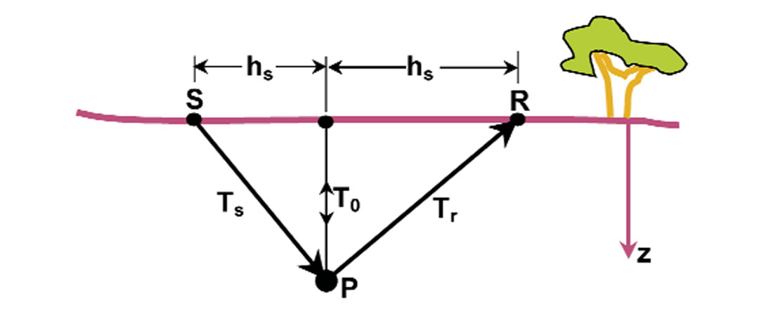
Figure 1 shows a source and receiver raypath with displacements h_s and h_r from the surface location of a scatterpoint, and with corresponding traveltimes T_s and T_r. The vertical two-way traveltime is defined by T₀ as in the zero offset case. I repeat for emphasis, that the velocity used for NMO correction, or source or receiver traveltimes for a Kirchhoff time migration, is computed using the RMS velocity that is defined at the scatterpoint.

The travel time for the source ray T_s is computed using the triangle containing the source ray and the half the zero-offset time T₀/2 giving

and similarly the traveltime for the receiver ray T_r is computed with

The total travel time T=T_s + T_r becomes

which is usually referred to as the double-square-root (DSR) equation. It is this equation that defines the traveltimes for any source or receiver to one scatterpoint.

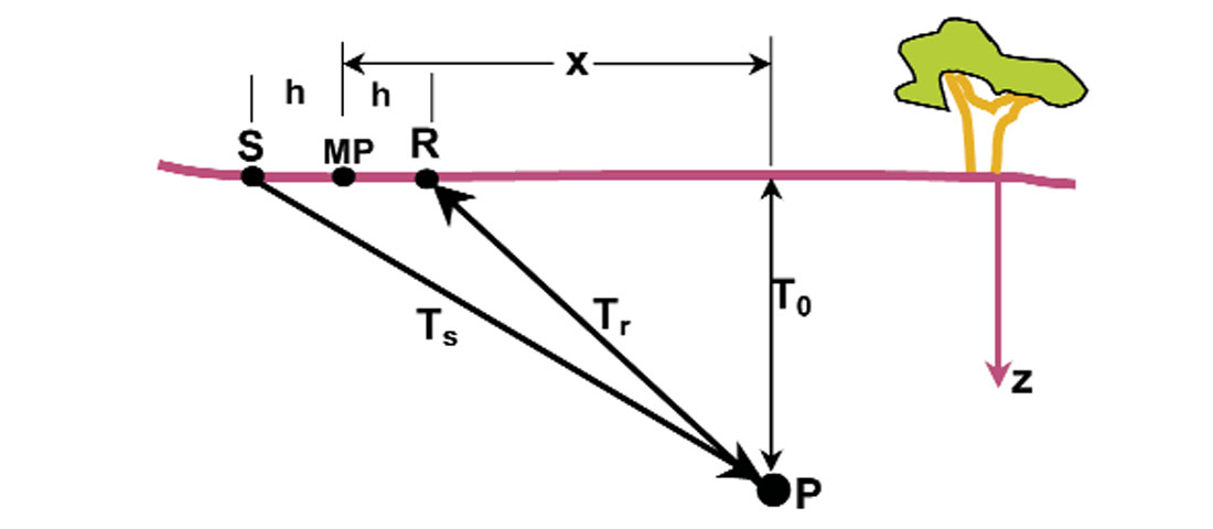
When we only have one scatterpoint, it is convenient to define the origin at the surface location of the scatterpoint and define an input trace by its relative midpoint location. We therefore write equation for the geometry in Figure 2, defining the surface distance from the scatterpoint to the midpoint (MP) as x, and the distance from the midpoint to the source or receiver as h, i.e.

Moveout correction for a dipping reflector

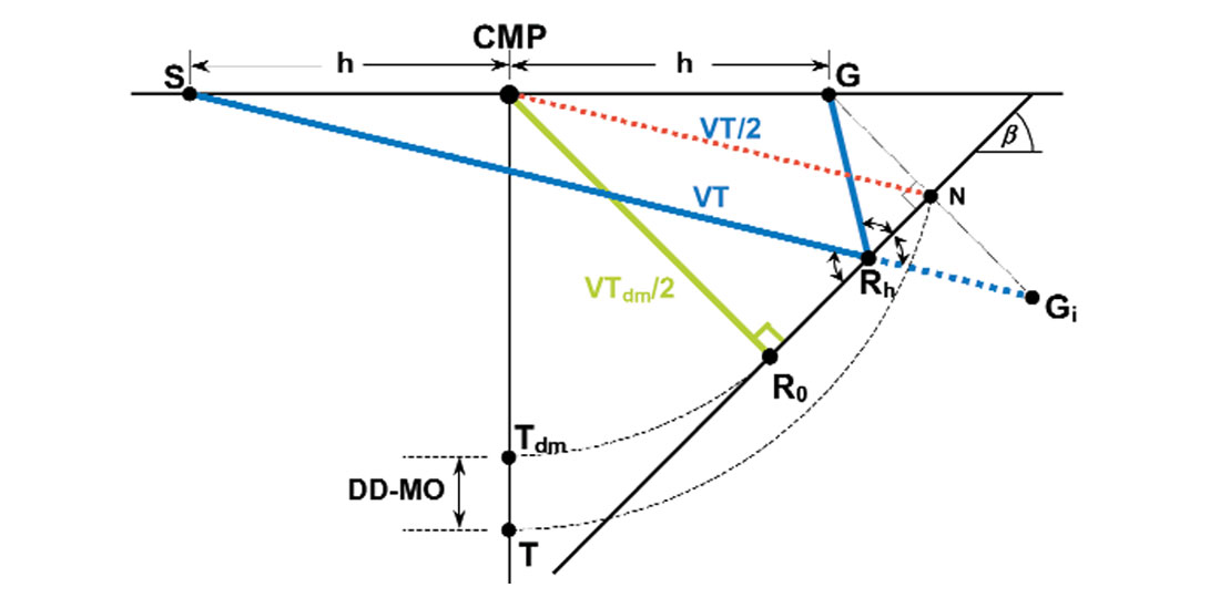
Even though the DSR equation is slightly complex for a scatterpoint, the moveout for horizontal or dipping linear reflectors, in a constant velocity medium, is exactly hyperbolic. Normal moveout may be applied to a common midpoint (CMP) gather to flatten the reflection energy by using stacking velocities. This simplicity is derived using a reflector with dip β shown in Figure 3 along with two raypaths that have a CMP. The green raypath has a colocated source and receiver at CMP with a reflection point R_o, while the blue raypath has a source at S and receiver at G with half offset h, and its reflection point at R_h.

The location of the offset reflection point R_h can be found using the image of the receiver G_i about the dipping event. The length of the offset raypath S-R_h-G is equal to the direct distance S-G_i. Half of this distance is defined by CMP-N identified by a red dashed line, and may be proved by considering the similar triangles (S, R_h, G) and (CMP, N, G). In a constant velocity medium V, the offset travel time T may be used to define the length of the raypath, i.e. S-G_i = VT, and the corresponding half distance by CMP-N = VT/2. Similarly the length of the zero-offset raypath is CMP-R₀ = VT_dm/2. These two times are plotted on the trace below CMP with the appropriate time scale. (One might expect the symbol T₀ to be used in place of T_dm; however T₀ is reserved for the vertical zero-offset time as used in the first three equations.)

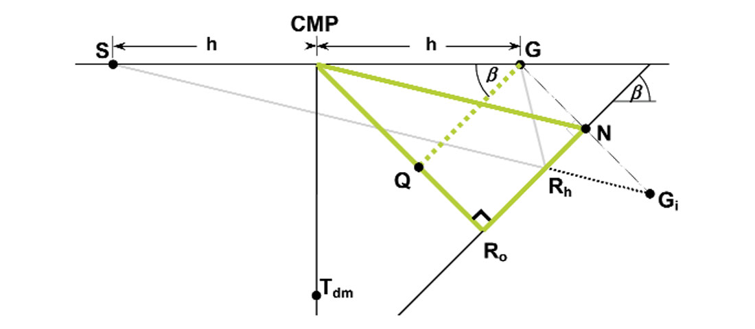
It is the objective of moveout correction to shift energy on the CMP time trace from time T to the zero-offset time T_dm. I will refer to this type of moveout for a dipping reflector as dip-dependent moveout (DD-MO). DD-MO is computed using features extracted from Figure 3a and highlighted in Figure 3b. Note the triangle (CMP, R₀, N) has two sides defined by the zero offset and offset traveltimes. The third side R₀-N is equal to the line Q-G that has the same geological dip β. The length of this line is defined using the triangle CMP-Q-G and is given by

The three sides of the triangle are related by the Pythagorean theorem giving

Expressing this equation in familiar form we get

in which we now define the stacking velocity V_stk to be

The right side of equation (2.7) is hyperbolic and applies for any CMP location, or for any half-offset h. This result is very significant and tells us that even for a constant velocity medium with a dipping reflector:

• the moveout is exactly hyperbolic for all traces in a CMP gather, and that
• dip-dependent moveout (DD-MO) correction requires a higher velocity V_stk.

This result may appear to be an ideal solution that simplifies seismic processing, however there is one major problem: the location of the reflection points. Note that the offset reflection point R_h is updip from the zero offset reflection point R₀. In fact, all traces in the same CMP gather will have reflection points that move up dip with increasing offset. DD-MO and stacking of this dipping reflection energy in a CMP gather will therefore smear the energy along the dipping reflector. We will see in a later section that, for a given reflection point on a dipping reflector, we must gather the energy from a path in the prestack volume that moves down dip as the half-offset h increases.

Typical of geophysical practice, equation (2.8) is extended to include RMS velocities giving

The stacking velocity V_stk is usually reserved for the moveout correction of dipping events, and the RMS velocity V_rms for the moveout correction of horizontal events and for migrations. (This means that we now use the RMS velocity for the best hyperbolic fit to the diffraction rather than the more formal definition that matches the moveout curvature at zero offset.)

A seismic data processor automatically picks the stacking velocity Vstk when flattening NMO corrected reflections in a CMP gather, and may be unaware that they are higher than V_rms when stacking dipping events. This creates a potential problem when estimating interval velocities for geological continuity or for migrating data. These processes expect RMS velocities and will produce errors in structured areas if V_stk is used. Therefore, a process that converts stacking velocity V_stk into RMS velocities V_rms, using equation (2.9), should be used when processing structured data.

Prestack volume P(x, h, t) for 2D data

Poststack data assume the source and receiver are colocated or are at the same position. Prestack data assumes that there is a finite distance 2h between the source and receiver. The half-offset parameter h could be a vector that includes direction, however, for 2D data that is acquired in a single line on the surface, h can be simplified to a positive or negative value. The inclusion of h adds another dimension to the input data creating three-dimensional prestack data P(x, h, t) for a 2D line. Similarly, 3D data becomes four dimensional in prestack P(x, y, h, t). The prestack volume for 2D data P(x, h, t) is illustrated in Figure 4a, showing the location of a zero-offset trace in green and a small-offset trace in red. Only the positive range (or possibly the magnitude) of h is shown, with zero-offset on the front face of the volume. Note the three equal distances identified by h around the CMP location.

For a 2D seismic line, the volume is filled with traces and there are a number of ways to organize this input data such as source (or shot) records, constant offset sections, or common midpoint gathers. These three arrangements of 2D data are illustrated in Figures 4b, 4c, and 4d. The shot record in Figure 4b contains blue traces along a line that is 45 degrees to the zero offset plane. The receivers are to the left of the source with a both a CMP location and offset equal to h. A selection of data at a constant offset is illustrated in part (c) and a CMP gather in part (d).

Specular energy from horizontal and dipping reflectors in the prestack volume

A horizontal reflector in a constant velocity medium V is illustrated in the prestack volume shown in Figure 5a. The vertical time scale is plotted with the zero-offset two-way time that is equal to the depth of the reflector. The horizontal reflector and zero-offset reflection are shown coincident on the front surface with zero-offset (h=0) and time T₀. The two-way travel time T of the specular (or mirror like) energy for offset data forms a hyperbolic cylinder (variations with h but not in x), with moveout that is exactly hyperbolic as defined by the normal moveout equation

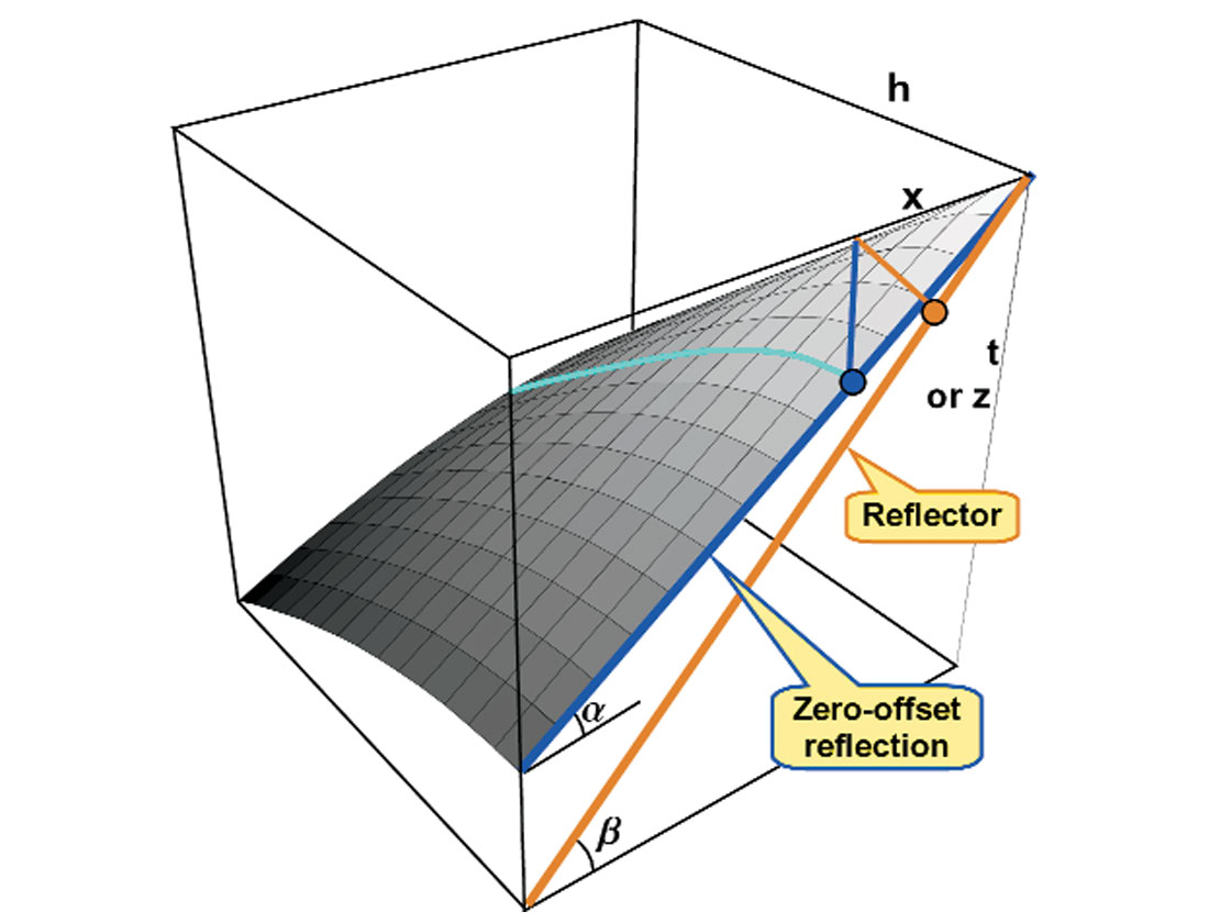
A dipping reflector and its prestack reflection in a constant velocity medium V are shown in Figure 5b, also with the vertical time scale that matches two-way time with depth. The dipping reflector with dip β is shown in brown, and the corresponding zero offset reflection in blue with dip. A zero-offset raypath that is normal to the reflector is shown in brown, along with its corresponding vertical time in blue, which is located on the zero offset reflection. A post-stack migration would move energy from the location at this time point to the corresponding location on the dipping reflector. The move out for a dipping reflector has been defined by equation (2.7) and is also exactly hyperbolic for a CMP gather as illustrated by the light blue curve, however, the hyperbolic shape is defined by the stacking velocity that was defined in equation (2.8). It may appear that conventional processing of moveout correction, stacking, and poststack migration would gather the energy reflected from the point on the reflector. That is not the case as the offset-reflected energy in the CMP gather comes from points up dip from the zero-offset reflection point as described above. The actual location of energy from the reflector point will be described in a following section.

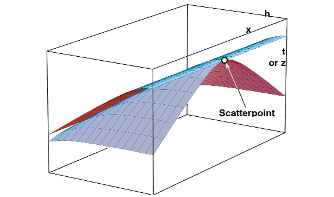
A scatterpoint’s reflection in the prestack volume

We will now use the double-square-root equation (2.4) to define a traveltime surface from one scatterpoint within the prestack volume P(x, h, t). This surface is displayed in Figure 6 with parts (a) and (b) showing front and rear views. Since its shape resembles the rounded pyramid on the Gaza plateau in Egypt, it is referred to as Cheops pyramid. Only half of the pyramid is displayed by using only positive values for h. There are a number of highlighted curves on the pyramid’s surface. The orange curve in Figures 6a and 6b represent the zero offset hyperbola that may be found when h=0 in equation (2.4), i.e.,

giving the kinematic equation of a diffraction for a poststack Kirchhoff migration operator.

The black curve in Figure 6b represents the single CMP gather that passes through the scatterpoint, where the displacement x is zero, giving the normal moveout equation (2.10), i.e.

The red curve represents all the other CMP gathers that do not pass through the scatterpoint. These curves are not hyperbolic and conventional moveout correction will not allow all the energy to stack at the desired zero-offset location, i.e. diffractions don’t stack, even in a constant velocity environment. At zero offset, the curvature of this red curve matches the curvature of a DD-MO hyperbola that uses the seismic dip (x) on the zero-offset diffraction to estimate the stacking velocity V_stk. This curvature matching at small offsets is one reason why offset-limited seismic processing has been successful in areas with dipping reflectors. In contrast, a prestack migration can include the larger offsets when using the DSR equation for improved processing.

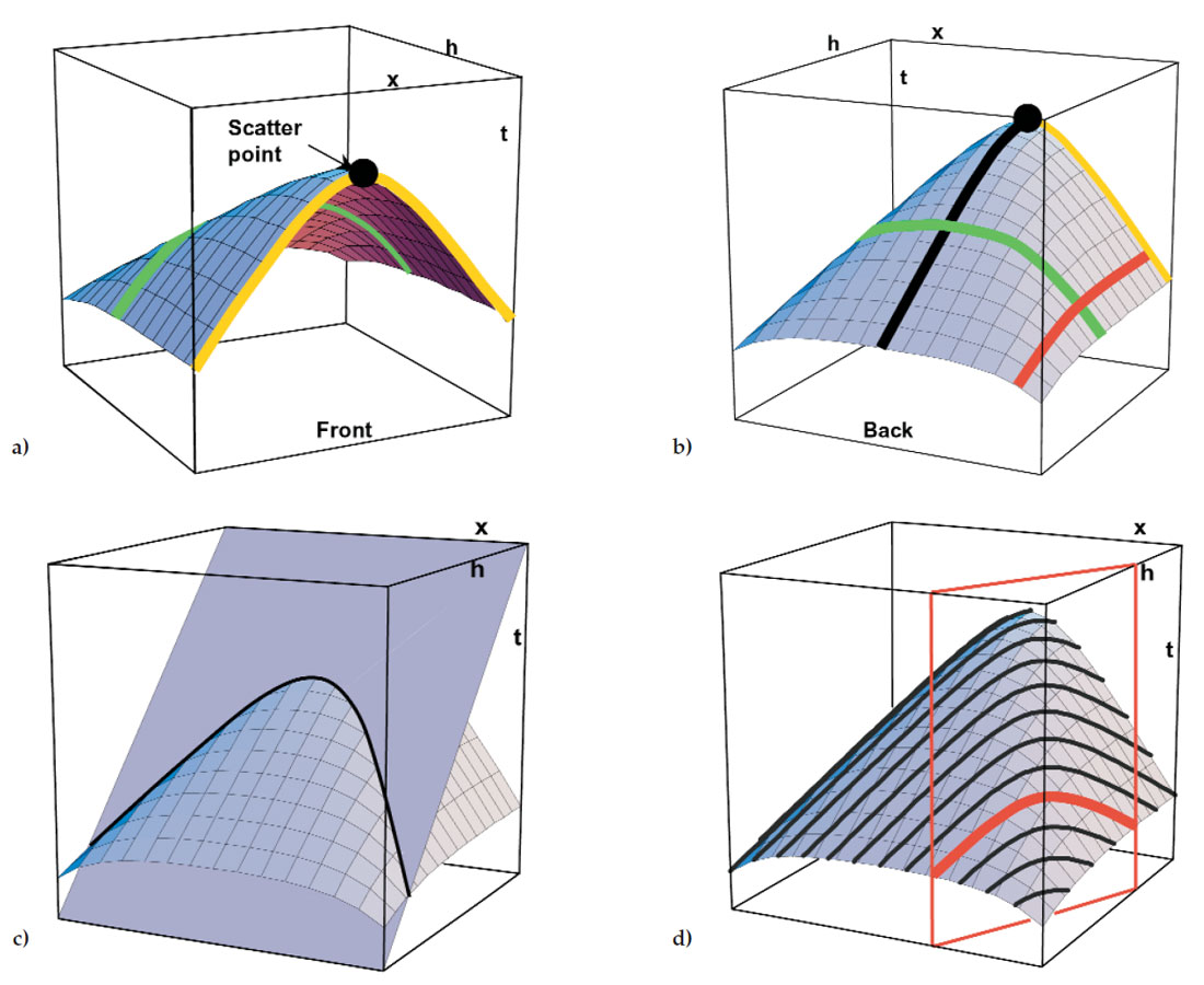
A constant offset diffraction is identified by the green curve. These curves are also non-hyperbolic, requiring the full DSR equation, and tend to be flatter at the apex.

Figure 6c shows the hyperbolic intersection of a radial plane through Cheops pyramid. This interesting hyperbolic feature has led to special prestack algorithms that include radial plane migrations and migrations in the tau-P space. Figure 6d shows the intersection of vertical planes, at 45 degrees to zero offset, which represent source gathers. The intersection of these vertical planes with Cheops pyramid define the shape of diffractions on the source gathers. It is interesting to note that all these diffractions have the same hyperbolic shape.

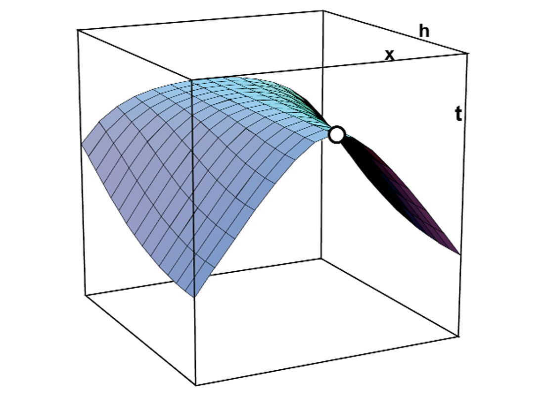
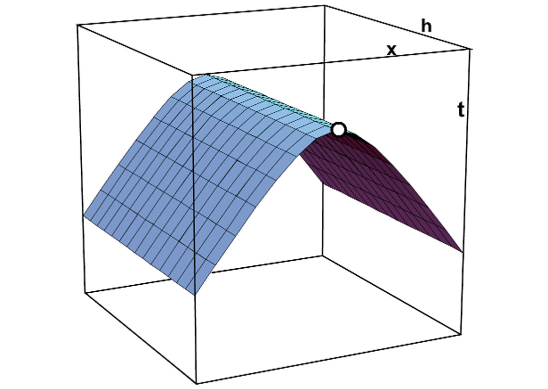
Figure 7a shows the effect on the traveltime surface when conventional NMO correction is applied to the traveltimes defined by Cheops pyramid. Figure 6b shows the desired traveltime correction, which has the same hyperbolic traveltimes at all offsets. Stacking, or summing this energy in Figure 6b to zero offset will produce the maximum energy on the zero offset diffraction, ready for poststack migration. The prestack process of dip moveout (DMO) converts energy from the shape in Figure 7a to the hyperbolic cylinder shape in Figure 7b.

Modelling with Cheops pyramid

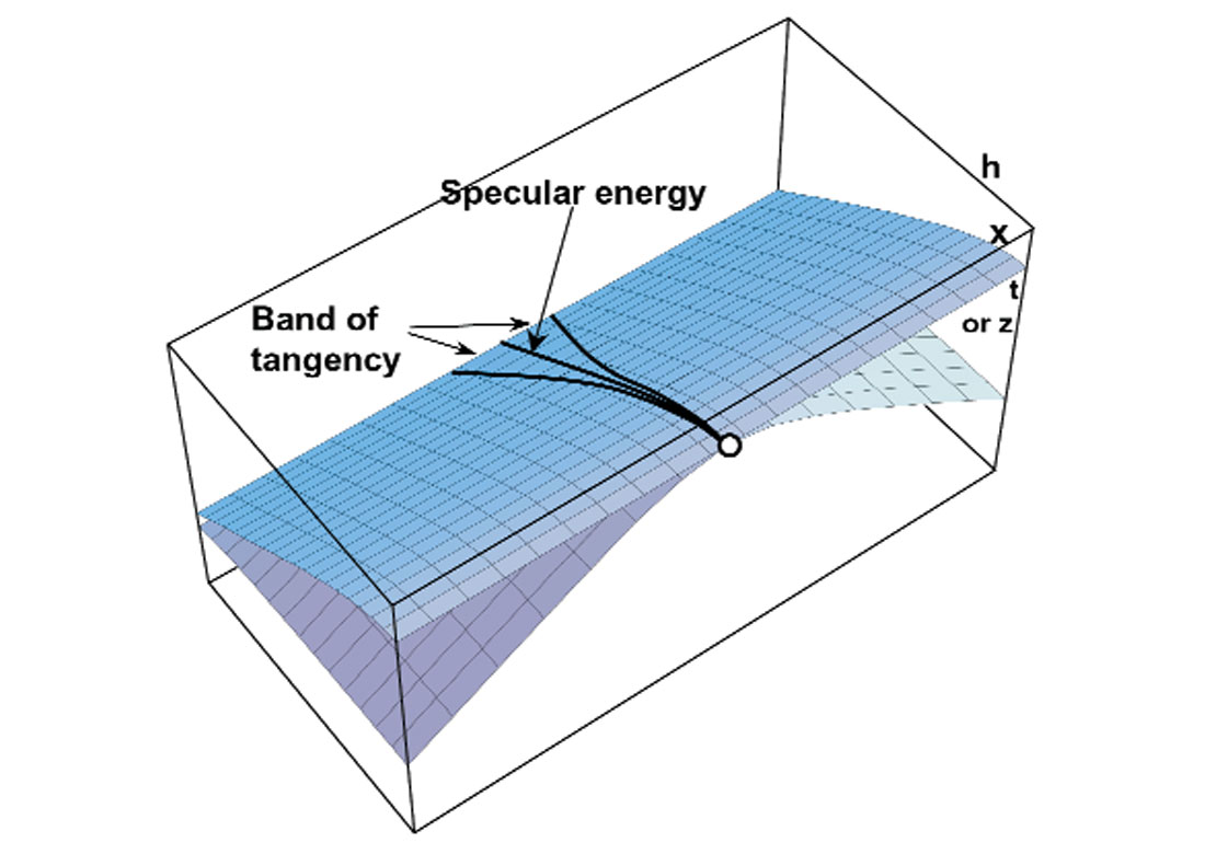
In the first article of this series I demonstrated diffraction modelling in which the energy of each point on the geological cross-section (all possible scatterpoints) is spread along its corresponding diffraction curve. We can accomplish the same task in the prestack volume by extending the zero-offset diffraction to include all offsets of the corresponding Cheops pyramid. Consider the horizontal reflector in Figures 8a and b. Each scatter point along the reflector becomes a Cheops pyramid (only one shown) and the hyperbolic surface is constructed, while the energy below this surface is destructively cancelled. The construction and cancellation of this energy is dependent on the trace spacing, velocity, and frequency content.

Each Cheops pyramid will have a band of tangency with the hyperbolic reflection surface as illustrated in Figure 8b.

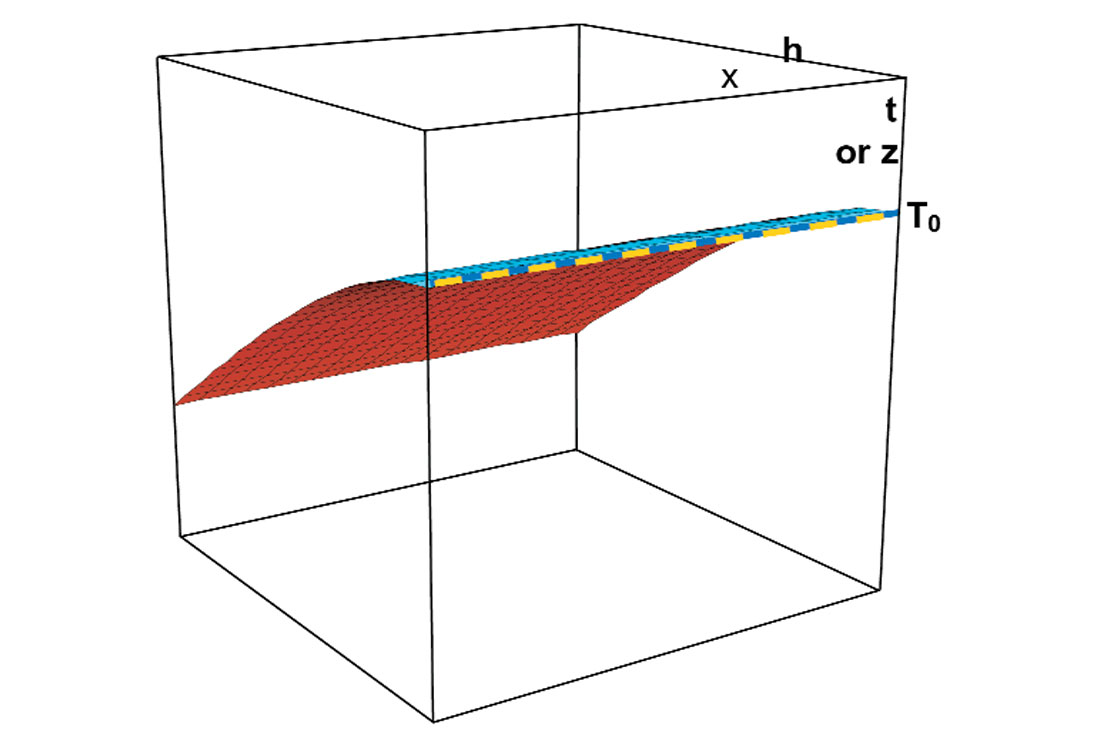
The modelling of a dipping reflector is illustrated in Figure 9 where the dipping reflector is shown in red on the zero-offset surface, and the zero offset reflection in blue. One scatterpoint on the dipping event and its corresponding zero offset location is also shown. Once again each point on the dipping reflector is modelled with a Cheops pyramid (only one shown in light gray) to reconstruct the prestack reflection surface. We have already shown that the dipping reflector surface (in dark gray) is exactly hyperbolic in the CMP gathers. However, the reconstruction of energy is not along the CMP gathers of the yellow dashed line, but along the line of tangency with Cheops pyramid as identified by the green line, which moves down dip as the offset is increased. This specular energy from the dipping reflector lies along the band of tangency that surrounds the green line. All other energy on Cheops pyramid that is below the reflection surface will destructively cancel.

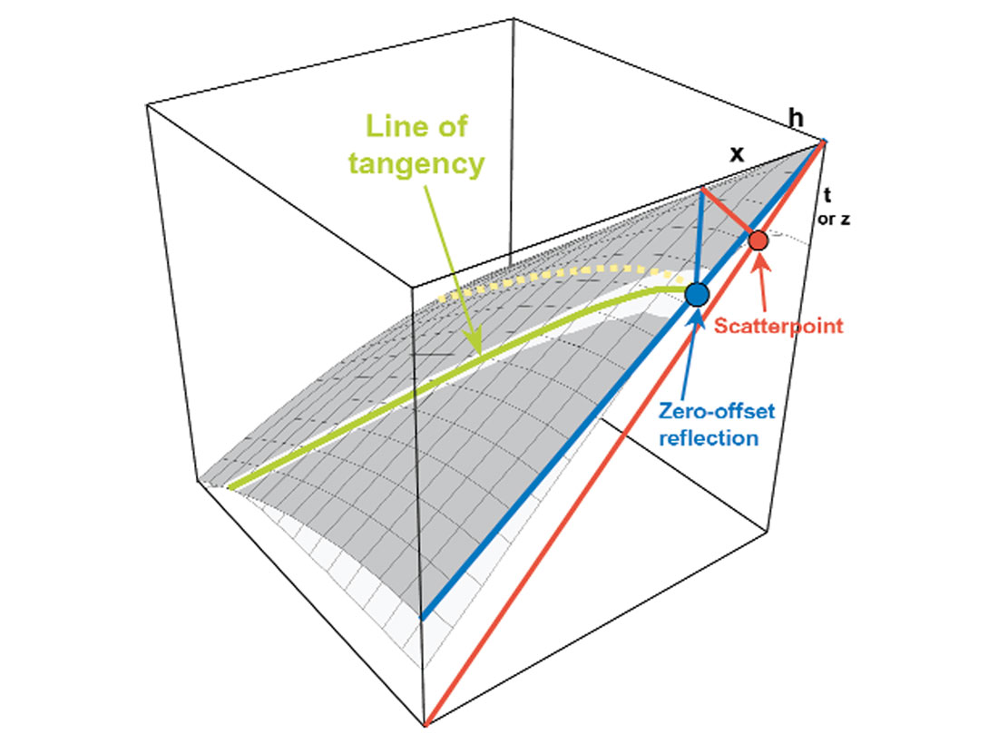
As in the poststack case we reverse the prestack modelling procedure to perform the prestack migration. Note in Figure 9 that the desired specular prestack energy that should be summed to the scatterpoint lies along the band that surrounds the green line of tangency.

Diffractions on a source gather

Consider the geometry of one source and a continuum of many receivers on the surface above a single scatterpoint as illustrated in Figure 10. This diagram is plotted with two-way time and with the “traces” below the surface location of the receiver (not at the CMP location). Assume the velocity is unity and that time is represented by distance. The travel time of the scatterpoint diffraction is the sum of the source ray travel time T_s (in red) and the receiver ray traveltime T_r (in blue). Note that T_s is always constant and independent of the receiver ray path. The shape of the diffraction is entirely due to the traveltime of rays from the scatterpoint to the receivers. Changing the relative location of the source will alter the vertical location of the diffraction but not its shape.

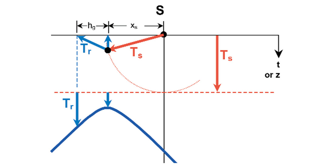
Figure 11 shows many scatterpoints that are located at the same depth, and their corresponding diffractions. Note that all diffractions have the identical shape, and that the distance from the source to the scatterpoint determines the vertical position of the diffractions. An interesting observation on this figure is that the reflection energy from a horizontal reflector will be the envelope of the individual scatterpoint diffractions.

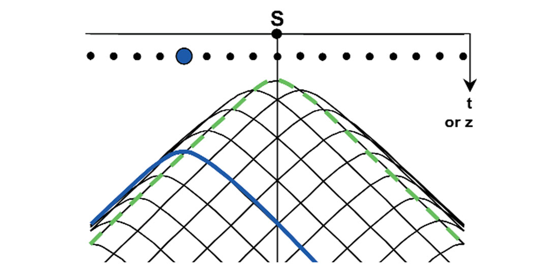
In Figure 11, there is one source and a continuum of receivers on the surface that are above a number of scatterpoints that are at the same depth. A similar image could also be created from one receiver and a continuum of sources along the surface to form a (common) receiver gather. Also note the similarity to Figure 6d that contains one scatter point and a number of source gathers that intersect Cheops pyramid, all with the same diffraction shape.

Diffraction on a constant offset section

Figure 12 represents a constant offset section in which all traces have the same the source-receiver offset defined by the distance 2h. The figure contains one scatterpoint and the kinematics of its offset diffraction shown in red. For reference purposes, a zero offset diffraction is shown in blue.

At large displacements x from the scatterpoint, the offset diffraction tends to the zero offset diffraction. At small displacements, the offset diffraction tends to flatten with its apex below the scatterpoint. This offset diffraction shape is defined by the DSR equation and is similar to the green line on Cheops pyramid in Figures 6a and 6b. NMO correction would move the apex of the offset diffraction to the apex of the zero offset diffraction, however all other points would move to times less than the zero-offset diffraction as indicated in Figure 7a.

The energy in a constant offset section is not easily created by using the exploding reflector model and is not easily migrated with a downward continuation process. However modelling and migration are very easily accomplished using the scatterpoint and diffraction concepts.

Prestack Migration Algorithms

Brute force Kirchhoff

If the input data were acquired with a sufficiently long recording time, energy from one scatterpoint could be found in every input trace. A brute force method of Kirchhoff migration could start by defining a single migration point with its vertical zero-offset time T₀, and then searching through all the input traces to find that energy that is located at the time defined by the DSR equation, then weighting and summing the energy back to the scatterpoint. This procedure would be repeated for all points in the migrated output section.

A more efficient method might consider all the scatterpoints in a migrated trace (or group of migrated traces) and then search through the input traces for the appropriate energy. The efficiency is improved when there is a maximum recording time that limits the range of input traces to some practical migration aperture, or when some type of dip limit is imposed.

Prestack Kirchhoff migration is based on the scatterpoint principle that assumes reflectors may be defined by scatterpoints, and that prestack seismic data becomes the superposition of the corresponding Cheops pyramids; i.e. summing over the Cheops pyramids to relocate energy back to the scatterpoints. However, the actual specular reflection energy lies on a prestack surface, and only the energy that is tangential to the Cheops pyramid is summed to the scatterpoint. Since the computer algorithm doesn’t know where the reflecting surfaces are, all possible surfaces are summed, i.e. all of Cheops pyramid is used. It is assumed that the sum of the specular energy in the area of tangency exceeds that of any noise summed over the remaining surface of the pyramid. True diffracted energy, such as that produced by a fault, will have energy spread over a larger area and will use more area on the summation surface of Cheops pyramid.

There are some migration algorithms that estimate the geological dip, and limit the range of summation to an area close to the assumed area of tangency. These algorithms may run faster and have a better signal-to-noise (SNR) than the more general algorithms. However, they must be used with care, as errors in the initial velocity model will tend to be “verified” by the migrated result.

Practical algorithms usually migrate data in either source gathers, common offset sections, or a combination of source and receiver gathers. These algorithms leave the data with some form of prestack offset that can then be used to evaluate and improve the velocity estimates or to provide amplitude versus offset (AVO) analysis.

Kirchhoff source gather migration

Direct Kirchhoff

The kinematics of a direct Kirchhoff migration of a source record are quite simple and similar to the poststack Kirchhoff migration; i.e. define a scatterpoint location, compute the diffraction shape, and sum the energy in the diffraction back to the scatterpoint. All that is required is to be able to define the diffraction shape that is identified in Figure 10 with traveltimes is computed by the DSR equation (2.13) that has been modified for the origin at the source location, with the distance to the scatterpoint x_s, and the diffraction offset h_g.

That’s all for the kinematics. The amplitudes need a little more work to take into account such things as the length of the source ray.

Combination of downward continuation and Kirchhoff

Another method of migrating a source gather combines a downward continuation process that collapses the shape of a diffraction, while a Kirchhoff type migration is used to compute the traveltime to the apex of the diffractions. Consider Figure 11 with many scatterpoints at a fixed depth. Downward continuing the source gather (with a conventional algorithm) to the depth of the scatterpoints, will collapse the diffraction energy to a point. For a time migration, that point will be at the apex of the diffractions, and is represented in the figure by the green dashed line. The time of this green line is computed using Kirchhoff concepts, which combine the traveltimes of the source ray and vertical receiver ray, for scatterpoints at the depth of the downward continuation. This time is often referred to as the imaging condition, or time where the migrated section is focused. A migration algorithm then maps the data at the imaging condition to the appropriate spatial position and the two-way time T₀ on the migrated section. For a depth migration, energy would be relocated to the scatterpoints.

Comments on the migration of source gathers

A source gather usually has a full complement of traces at all offsets and can be migrated with little concern of aliasing. However, energy from dipping or truncated events propagates beyond the boundaries of the original source gather to create larger offset traces. These larger offset traces may not represent the exact geological structure, but are required for its reconstruction when summed with other source records. It requires many source gathers to be summed to reconstruct the geological structure, and aliasing may occur if there are an insufficient number.

S-G method

The shot-geophone (S-G) method (we would now call it a source-receiver method), is based on a downward continuation method that alternates between the source and receiver gathers. In source gathers, the diffractions are defined by the depth of the scatterpoints relative to the receivers, and in receiver gathers, the diffractions are defined by the depth of the scatter points relative to the sources. By alternating the downward continuation (D-C) increments between the source and receiver gathers, the diffraction energy in both gathers will collapse towards the scatterpoints on the appropriate zero offset traces.

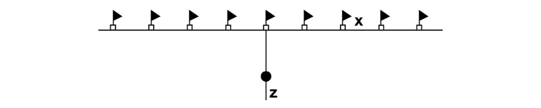
The alternating procedure of the S-G method is illustrated using Figures 13, 14, and 15. Figure 13 shows a simple geometry with sources and receivers at each station above a scatterpoint. Figure 14 shows source and receiver gathers with 14a showing the source gathers. These source gathers are D-C to the depth of the scatterpoint with one depth increment from the surface producing the source gathers in Figure 14b. The data are then sorted to receiver gathers in Figure 14c, where all the energy from the single scatterpoint, is collected into one receiver gather. These receiver gathers are then D-C to the depth of the scatterpoint, collapsing all the energy to one point as illustrated in Figure 14d.

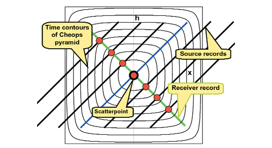
This same procedure is illustrated with Figure 15, which contains a plan view of Cheops pyramid. Plan views of source records are identified by the black lines that are at 45 degrees to zero offset. Also shown is one receiver gather identified by a green line, that is normal to the source lines. (The other receiver gathers would lie in a similar direction and pass through the zero-offset of the source records but are not shown.)

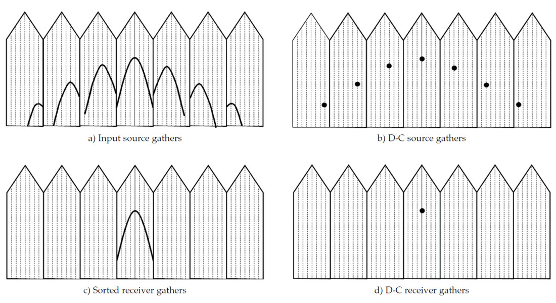
The single scatterpoint in Figure 15 produces identical diffraction shapes on all the initial source lines where they truncate Cheops pyramid. Downward continuing these source-gathers to the depth of the scatterpoint will move energy to the peak of the diffractions that are identified by the red dots, corresponding to Figure 14b. After sorting the data to receiver gathers, all the red dots lie on the one receiver line that passes through the scatterpoint at the apex of the pyramid corresponding to Figure 14c. Downward continuation of the receiver lines to the depth of the scatterpoint will also collapse the remaining diffracted energy to the apex of the diffraction that is at zero offset in both gathers. All the energy on the surface of Cheops pyramid is now focused to the one trace at the scatterpoint.

The normal D-C process is accomplished with many small depth increments, with the sorting between source and receiver gathers at each depth increment. In real data, the prestack volume is occupied by a very large number of Cheops pyramids, all of which, when downward continued to the appropriate depth, should focus to scatterpoints or reflectors on the vertical plane at zero offset. At each depth level, this focused energy is copied to the migrated section at the corresponding time or depth level. The accuracy of the velocity model controls how well the data focuses to the zero offset trace.

In a source gather the trace interval is defined by the incremental distance between the receivers, and in a receiver gather the trace interval is defined the incremental distance between the sources. The example illustrated above had a source at every receiver location and that produces an equal trace interval in both the source and receiver gathers. However, most 2D data is acquired with sources at multiple increments of the receivers, i.e. a source at every fourth receiver location. Now the receiver gathers have a much larger trace spacing that may produce aliasing problems. Practical applications may therefore require some form of trace interpolation to reduce the trace spacing in the receiver gathers.

The S-G method requires a tremendous amount of data sorting between source and receiver gathers. This sorting runs more efficiently on computers with a large “CPU” memory, and where the sorting of traces can become an addressing process in programming languages such as “C”.

Constant offset migration

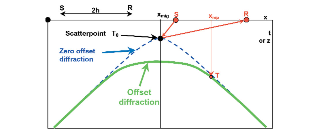
The migration of a constant offset section becomes a simple task when considering the diffraction illustrated by the green curve on Cheops pyramid in Figure 6b, or on the constant offset section in Figure 12. The traveltimes are defined by keeping the half-offset term h_c constant in the double square-root equation, i.e.,

Equation (2.14) is defined with the origin above the scatterpoint. When many scatterpoints define the geology, the origin can be placed at the left side of the section, then equation (2.14) may be written as

EQUATION 2.15

where x_mig is the surface location of the migrated trace, and x_mp is the surface location of the input trace. The migration aperture for one migrated sample at (x_mig, T₀) will cover the range defined by x_mig - x_mp and will have traveltimes T defined by equation (2.15).

A constant offset section usually has many missing traces and a number of constant offset sections may be summed with the appropriate differential moveout correction to form a limited offset gather. These limited offset gathers are then assumed to be constant offset sections with no missing traces, and can be migrated with a Kirchhoff algorithm to produce an image that is similar to the geological structure. Summing or stacking of all the migrated constant offset sections should create a geological structure that has an improved signal-to-noise ratio that is better than any single constant offset section.

Amplitude scaling along the diffraction is a complex issue that is still being evaluated in the current research literature of inversion. A simple but effective scheme would use the weightings similar to the zero-offset case.

Dip Moveout (DMO)

In a constant velocity medium, NMO correction, DMO, and poststack migration are equivalent to prestack migration. In very smoothly varying velocities, such as a marine environment, DMO can be more efficient than prestack migration and reduce runtimes. However, prestack time migrations are typically based on the RMS velocity assumption that has a more general application.

GDMO-PSI

Gardner’s method of applying dip moveout before NMO correction (GDMO) combined with the prestack imaging process (PSI) produces a potentially powerful prestack technique that produces prestack migration gathers with no velocity information. Reflection energy is confined to hyperbolic paths similar to the energy in a CMP gather. Analysis of these gathers produces accurate velocities, which are used to apply Kirchhoff NMO correction and stacking to complete the prestack migration. (Kirchhoff NMO correction implies that amplitude scaling and anti-aliasing filters accompany the moveout). The GDMO that is required for this process is expensive in computer runtimes, so approximations are used in commercial applications.

Equivalent offset method (EOM)

The equivalent offset method of prestack time migration is based on prestack Kirchhoff migration and the RMS velocity assumption. Mapping of scattered energy directly to the prestack migration gather is accomplished through a process that converts the DSR equation to a hyperbolic form. The prestack migration gathers, which are referred to as common scatterpoint (CSP) gathers, require no DMO and are formed with no time shifting of the input data. Accurate velocity information is extracted after the CSP gathers are formed and then Kirchhoff NMO and stacking complete the migration process. Since this method is based on Kirchhoff migration principles, arbitrary input geometries can be migrated to arbitrary migrated geometries. For example, a small window in a section, also known as a porthole, allows real-time interactive analysis of migration parameters such as the variation of dip limits, velocity tuning, or the effects of anti-aliasing filters. The prestack migration of various 3D projects acquired with different geometries and orientations may be accomplished without the need for re-gridding, or any arbitrarily located 2D line can be prestack migrated from a 3D volume of input data.

The basic prestack time-migration algorithm of EOM described above has been extended to prestack depth migrations that include anisotropy, migrations from a rugged surface elevation, the prestack migration of converted wave data, the prestack migration of borehole data, and the estimation of statics based on prestack migrated models of the source records.

Comparison of a poststack and prestack migration

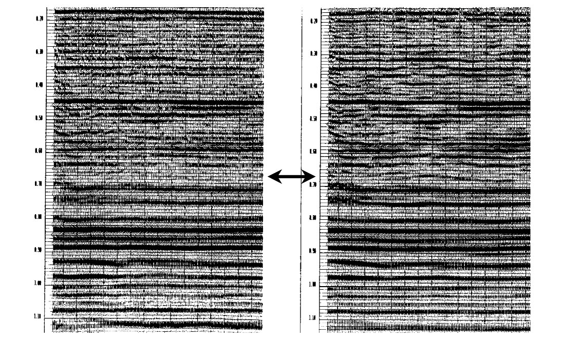
Figure 16 compares a poststack time migration with a prestack time migration using EOM on a data set that is essentially flat. The same single velocity function was used for both data sets. Note the anomaly, indicated at the time of the arrow, appears to be more evident on the prestack migration, illustrating the improved focusing that can be achieved with prestack migrations.

Conclusions

In a constant velocity medium, NMO correction is only valid for horizontal reflectors. With dipping reflectors, the moveout in a CMP gather is hyperbolic, however the energy comes from reflection points that move up dip, smearing events along the reflector. The moveout energy from a scatterpoint is non-hyperbolic and will not stack to the zero-offset hyperbola, i.e. diffractions don’t stack.

The correct focusing of energy requires a prestack migration process that assumes the prestack kinematic surface is defined by the DSR equation or has the shape of Cheops pyramid. There are many algorithms that achieve this objective such as the brute force Kirchhoff method, where all input data is summed directly to the migrated samples. Other algorithms migrate data in source gathers or constant offset sections, leaving the migrated data at some offset for additional processing, such as refined velocity analysis or amplitude versus offset (AVO) considerations.

Dip moveout (DMO) is a process that essentially performs a partial migration that maps offset energy to zero-offset, allowing a poststack migration to complete the prestack process. This method is much faster than true prestack migrations, but since it is based on constant velocity assumptions, its applications have been limited to areas with smooth velocity variations.

Some prestack methods form prestack migration gathers in which the reflected energy is located at offsets that represent the actual distance between the scatterpoint and the location of the source and receiver. This is in contrast to methods that migrate source gathers or constant offset sections that leave the prestack migrated data at an offset defined by the source-receiver half offset. Velocity analysis performed on gathers that uses the geometry of the raypaths rather than the source-receiver offset will converge more rapidly.

The next paper in this series

The first two papers in this series essentially address the kinematics of post- and prestack migration as described in my SEG course notes. The next paper will attempt to address some of the issues that involve amplitudes, starting with the method of diffraction stacking and matched filters, solutions to the wave-equation, and then the basic concepts leading to inversion.