Seismic Attributes – a promising aid for geologic prediction

Seismic attributes have come a long way since their introduction in the early 1970s and have become an integral part of seismic interpretation projects. Today, they are being used widely for lithological and petrophysical prediction of reservoirs and various methodologies have been developed for their application to broader hydrocarbon exploration and development decision making. Beginning with the digital recording of seismic data in the early 1960s and the ensuing bright spot analysis, the 1970s saw the introduction of complex trace attributes and seismic inversion along with their color displays. This was followed by the development of response attributes, introduction of texture analysis, 2D attributes, horizon and interval attributes and the pervasive use of color. 3D seismic acquisition dominated the 1990s as the most successful exploration technology of several decades and along with that came the seismic sequence attributes. The coherence technology introduced in the mid 1990s significantly changed the way geophysicists interpreted seismic data. This was followed by the introduction of spectral decomposition in the late 1990s and a host of methods for evaluation of a combination of attributes. These included pattern recognition techniques as well as neural network applications. These developments continued into the new millennium, with enhanced visualization and 3D computation and interpretation of texture and curvature attributes coming to the forefront. Of course all this was possible with the power of scientific computing making significant advances during the same period of time. A detailed reconstruction of these key historical events that lead to the modern seismic attribute analysis may be found in Chopra and Marfurt (2005). The proliferation of seismic attributes in the last two decades has led to attempts to their classification and to bring some order to their chaotic development.

We pick up the threads of this development over the last five to six years that has lead to the present seismic attribute analysis tools and workflows and also discuss some applications of seismic attributes that demonstrate the direction in which the attribute development is headed. Finally, a reasonable expectation is enunciated in that seismic attributes will continue to improve accuracy of interpretations and predictions in hydrocarbon exploration and development.

The 1990s saw 3D attribute extractions become commonplace in the interpretation work place. During this time seismic interpreters were making use of dip and azimuth maps, amplitude extractions and seismic sequence attribute mapping concepts were also established. Seismic coherence was introduced, which distinctly revealed buried deltas, river channels, reefs and dewatering features. The remarkable detail with which stratigraphic features show up on coherence displays, without any interpretation bias, and some unidentifiable even with close scrutiny, appealed to the interpreters and this has significantly changed the way geophysicists interpret 3D seismic data.

In 1999, Greg Partyka introduced the application of spectral decomposition to stacked seismic data. This allowed interpreters to utilize the discrete frequency components of the seismic bandwidth to interpret and understand the subtle details of subsurface stratigraphy. During the same year Connolly (1999) introduced elastic impedance, which computes conventional acoustic impedance for non-normal angle of incidence. Crossplotting of attributes was introduced to visually display the relationship of two or three variables (White, 1991). Such crossplots have been used since as AVO anomaly indicators (Hilterman and Verm, 1994). Automated pattern recognition on attributes through neural network applications, geostatistics and multivariant regression analysis have helped combine attributes sensitive to relevant geological features. Waveform classification schemes were introduced by Elf Acquitaine in the mid 1990s, where the interpreter defines a zone of interest pegged to an interpreted horizon, and then asks the computer to define a suite of approximately 10-20 waveforms that best express the data. Keeping pace with such emerging technologies were the advancements in visualization. Starting at the seed voxels, a seed tracker will search for connected voxels that satisfy the user-defined search criteria, thereby generating a 3D ‘geobody’ within the 3D seismic volume.

Significant developments: Recent past

Spectral decomposition

This work continues actively today, with most workers preferring the wavelet transform based approach introduced by Castagna et al. (2003) over the original discrete Fourier Figure 1. A time slice (a) at 2000 ms showing the channel as seen on the 3D seismic (b) 17 Hz amplitude slice from spec-transform.

Figures 1a and b show examples where the application of spectral decomposition on 3D seismic data from Southern Nigeria helped map the geometry of incised channels, one of the primary objectives of the study (Ojo and Sindiku, 2003). Conventional spectral decomposition (using Fourier Transform) was applied to 3D seismic data and viewed in map form. The spectral responses within the zone-of-interest showed the lateral variability of the channel complex clearly and indicated the fault trend as well, features not evident on the traditional time slices. An interesting fact that emerged out of this analysis was that both the time and depth maps generated for the channel bases and the isopach maps of the channel-fill thickness conform to the geometry as obtained from spectral decomposition.

Besides imaging the subsurface features, spectral decomposition also helps discriminate the most significant frequency content of a reservoir and so optimizes the seismic image for stratigraphic and/or DHI interpretation (Fahmy et al., 2005). Figure 2 shows a segment of a seismic section from a field in offshore West Africa.

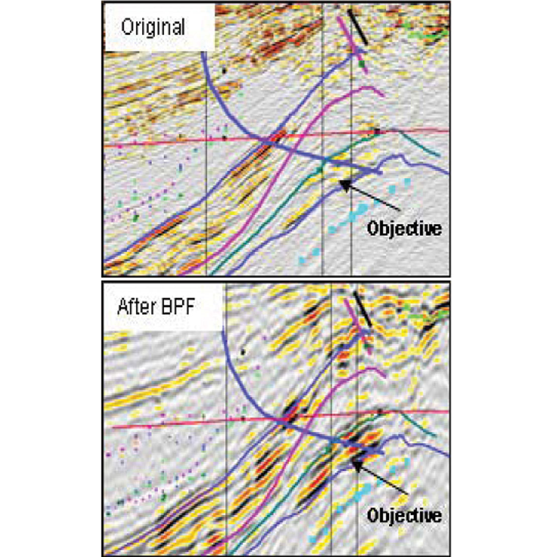
The discovery well drilled on this field encountered a 45 m net oil pay and a wet sand downdip by the sidetracked well. Another well was later proposed to prove the presence of a thicker reservoir updip, and evaluate its quality. However, since the seismic amplitude extraction did not support the presence of thicker or better quality sands updip from the first well, the drilling of this well was put on hold. Instantaneous spectral analysis was carried out on several seismic profiles that intersected the proposed well location. Analysis of the resultant frequency gathers showed that the majority of the signal’s strength for the reservoir reflections was confined to a narrow band of frequencies centered around 11 Hz and below 20 Hz. Consequently, a bandpass filter was designed and applied to the seismic data to preserve the signal bandwidth of the reservoir and attenuate all energy above 20 Hz. The resultant data showed lower resolution, but a pronounced low impedance anomaly corresponding to the reservoir showed up clearly. This significantly helped the interpretation of the stratigraphy from the seismic data. The well in question was later drilled and it encountered 154 m of net oil sands in the target reservoir, validating the pre-drill prognosis of better sand facies than the earlier well.

This example demonstrates the application of spectral decomposition for delineating a reservoir specific bandwidth and optimizing the seismic data for DHI and stratigraphic interpretation.

Spectral decomposition has been applied not only in the time domain, but in the depth domain as well. Montoya et al., (2005) demonstrate the application of spectral decomposition in the depth domain to an area in the Gulf of Mexico, which helped understand the distribution and classification of deep-water geological elements.

Seismic inversion revisited

The original recursive or trace-integration seismic inversion technique for acoustic impedance also evolved during the late 1980s and 1990s, with developments in model-based inversion, sparse-spike inversion, stratigraphic inversion, and geostatistical inversion, providing accurate results (Chopra and Kuhn, 2001). The earlier techniques used a local optimization method that produced good results when provided with an accurate starting model. Local optimization techniques were followed by global optimization methods that gave reasonable results even with sparse well control.

Connolly (1999) introduced elastic impedance, which computes conventional acoustic impedance for non-normal angle of incidence. This was further enhanced by Whitcombe (2002) to reflect different elastic parameters such as Lamé’s parameter λ, bulk modulus κ, and shear modulus μ.

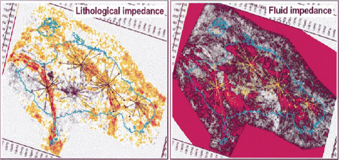
Figure 3 shows maps of average ‘extended elastic impedance’ averaged over a 25 ms time gate measured from top reservoir for the Forties field in the central North Sea. The images are tuned to shear and bulk modulus. These images show the ‘clear imaging of the channel systems and, potentially, remaining hydrocarbons within these channels’.

Crossplotting of attributes

Crossplotting of attributes was introduced to visually display the relationship between two or three variables (White, 1991). Hilterman and Verm (1994) used crossplots in AVO analysis, which have been used since as AVO anomaly indicators. When appropriate pairs of attributes are cross-plotted, common lithologies and fluid types often cluster together, providing a straightforward interpretation. The off-trend aggregations can then be more elaborately evaluated as potential hydrocarbon indicators, keeping in mind the fact that data that are anomalous statistically are geologically interesting - the essence of successful AVO crossplot analysis. Extension of crossplots to three dimensions is beneficial as data clusters ‘hanging in 3D space’ are more readily diagnostic, resulting in more accurate and reliable interpretation.

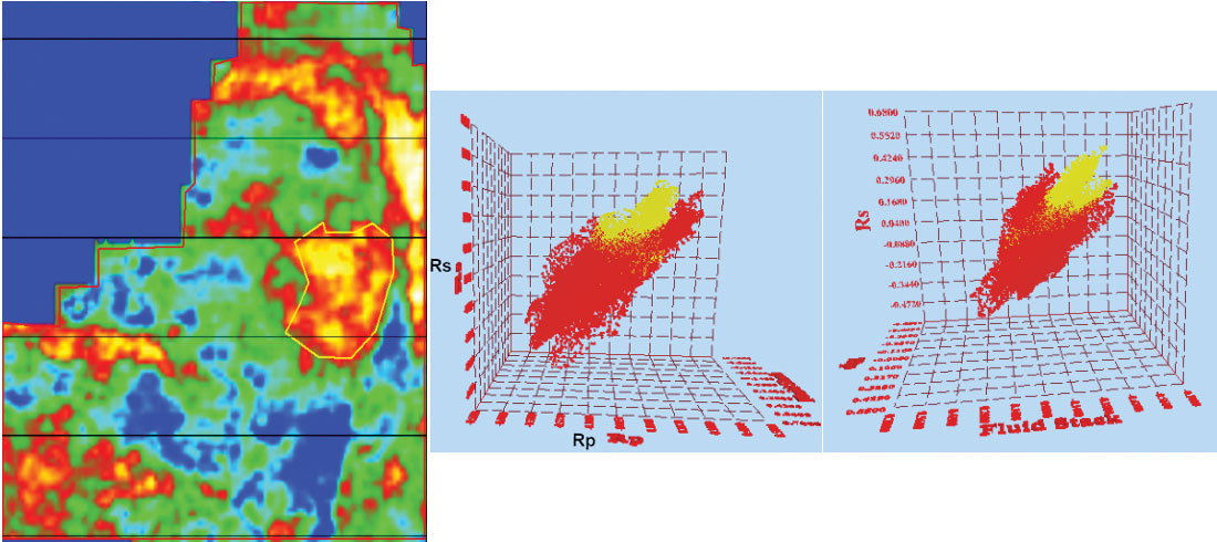
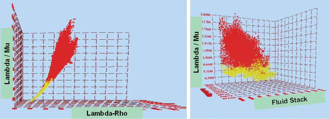
In Figure 4 we illustrate the use of modern crossplotting software of three attributes that help identify a gas anomaly – P-reflectivity on the x-axis, S-reflectivity on the y-axis and fluid stack on the z-axis. In Figure 4a, we indicate a gas anomaly on a time slice through the P-reflectivity volume by a yellow-red patch. We then draw a yellow polygon on the time slice to select live data points pertaining to the anomaly to be displayed in the crossplot. The red cluster of points in Figure 4b corresponds to the red polygon on the time slice (enclosing the live data points). As the crossplot is rotated toward the left on the vertical axis, the fluid stack shows the expected negative values for the gas sand (Figure 4c). In Figure 5 the AVO attribute Lambda-Rho, Lambda/Mu and Fluid stack are crossplotted. On the Lambda-Rho - Lambda/Mu crossplot the anomaly is seen as yellow cluster showing low values of Lambda-Rho and Lambda/Mu. As the crossplot is turned on the vertical axis, the fluid stack indicates negative values corresponding to the low values of Lambda-Rho and Lambda/Mu, indicating the gas sand clearly.

Automated pattern recognition on attributes

The attribute proliferation of the 1980s resulted in an explosion in the attribute data available to geophysicists. Besides being overwhelming, the sheer volume of data defied attempts to gauge the information contained within those data using conventional analytical tools, and made their meaningful and timely interpretation a challenge. For this reason, one school of geophysicists examined automated pattern recognition techniques, wherein a computer is trained to ‘see’ the patterns of interest and then made to sift through the available bulk of data seeking those patterns. A second school of geophysicists began combining attributes sensitive to relevant geological features through multi-attribute analysis.

Neural network application for multi-attribute analysis

One attempt at automated pattern recognition took the form of neural networks (Russell et al., 1997), wherein a set of input patterns is related to the output by a transformation that is encoded in the network weights. In Figure 6 we show an example on how multivariate statistical analysis can be used in determining whether the derived property volumes are related to gas saturation and lithology (Chopra and Pruden, 2003). For the case study from southern Alberta, it was found that the gamma ray logs in the area were diagnostic of sands, and there was a fairly even sampling of well data across the field. A non-linear multi-attribute determinant analysis was employed between the derived multiple seismic attribute volumes and the measured gamma ray values at wells. By training a neural network with a statistically representative population of the targeted log responses (gamma ray, sonic, and bulk density) and the multiple seismic attribute volumes available at each well, a non-linear multi-attribute transform was computed to produce gamma ray and bulk density inversions across the 3D seismic volume.

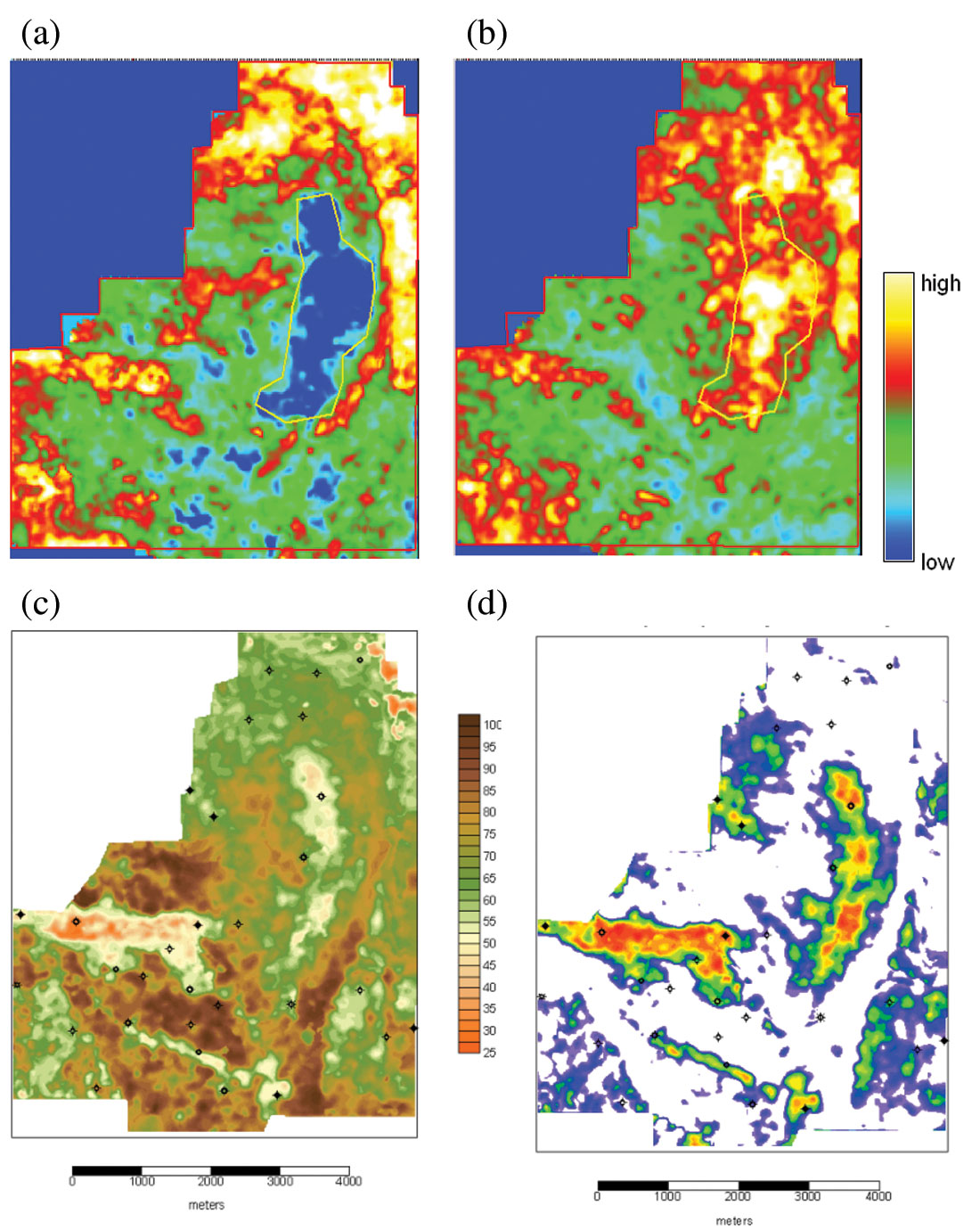
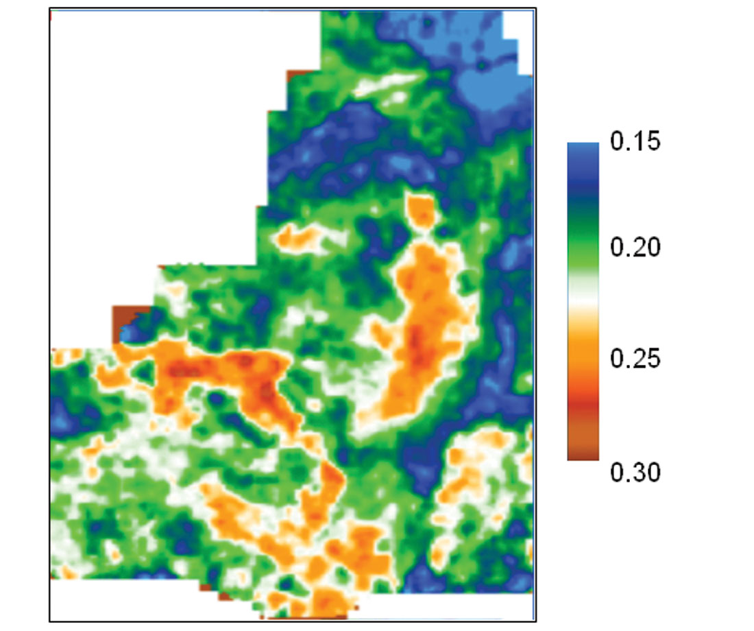
In Figures 6a and b we show the Lambda-Rho and Mu-Rho sections with the anomaly enclosed in a yellow polygon. Probabilistic neural network solutions were used to derive gamma inversion and are shown in Figure 6c. The data are scaled to API gamma units in Figure 6c and converted to porosity in Figure 6d using the standard linear density relationship. From log data, the sand filled channels are interpreted as having gamma values less than 50 API units. This cut off value was used to mask out inverted density values for silts and shales. Analysis of Figures 6c and d shows three distinct sand bearing channels. Cubic B-spline curves (mathematical representation of the approximating curves in the form of polynomials) have also been used for determination of mathematical relationships between pairs of variables from well logs and then using them to invert attribute volumes into useful inversion volumes like gamma ray and porosity (Chopra et al., 2004). In Figure 7 we show spline curve inverted porosity. Notice that the results from the cubic B-spline inversion and the neural network analysis look similar. It may be mentioned that the results could differ significantly if there is a significant variation in geology laterally, in which case the single well used for the spline analysis is no longer representative of the entire area.

Enhanced visualization helps attribute interpretation

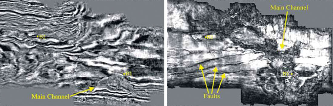
Gradually as geophysicists realized that the additional benefits provided by 3D seismic were beneficial for stratigraphic interpretation of data, seismic interpretation methods also shifted from simple horizon-based to volume-based work. This provided interpreters new insights that were gained by studying objects of different geological origins and their spatial relationships. In Figure 8 we display strat cubes (sub-volumes bounded by two not necessarily parallel horizons), generated from the coherence volumes. The coherence strat cube indicates the N-S channel very clearly, the E-W fault on the right side as well as the down thrown side of the N-S fault on the left.

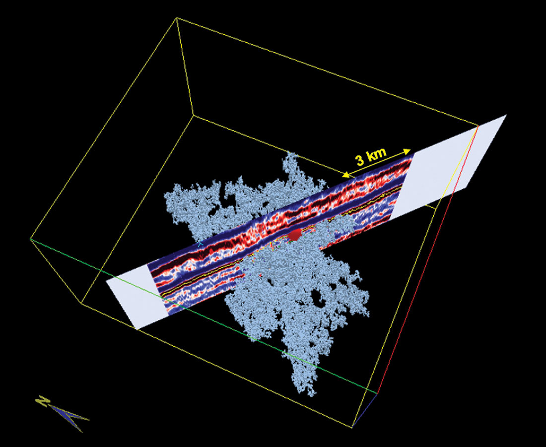
Of course with all this also came the complexity and the magnitude of identification work and the need for faster and more accurate tools. This brought about the significant introduction of techniques for automated identification of seismic objects and stratigraphic features. Geobody tracking is now possible by selecting an amplitude value corresponding to a feature of interest and letting the ‘seed tracker’ search for connected voxels that satisfy a user-defined search criterion. Complete geobodies corresponding to a porous sand accumulation, or a salt body or the channel-fill within a drainage system can be conveniently determined. Figure 9 shows the geobody-tracking of a porous zone in 3D space by selecting a seed amplitude at the point indicated by the small re d sphere. Such geobody-tracking helps in assessing the hydrocarbon reserves in place in a given prospect.

While one given attribute will be sensitive to a specific geologic feature of interest, a second attribute may be sensitive to a different kind of feature. We can therefore combine multiple attributes to enhance the contrast between features of interest and their surroundings. Different methodologies have been developed to recognize such features. Meldahl et al. (2001) used neural networks trained on combinations of attributes to recognize features that were first identified in a seed interpretation.

The network transforms the chosen attributes into a new ‘meta-attribute’, which indicates the probability of occurrence of the identified feature at different seismic positions. Such highlighted features definitely benefit from the knowledge of shapes and orientations of the features that can be added to the process.

Trace shape

While spectral decomposition and wavelet analysis compare seismic waveform to precomputed waveforms (typically windowed tapered sines and cosines), an important development was released by Elf Acquitaine in the mid 1990s – trace shape classification. In this approach, the interpreter defines a zone of interest pegged to an interpreted horizon, and then asks the computer to define a suite of approximately 10-20 waveforms that best express the data. The most useful of these classifiers is based on Self-Organized Maps (Coleou et al., 2003) that provides maps whose appearance is relatively insensitive to the number of classes. Although the results can be calibrated to well control through forward modeling, and although actual well classes can be inserted, this technology is particularly well suited to a geomorphology driven interpretation, whereby the interpreter identifies depositional and structural patterns from the images and from these infers reservoir properties.

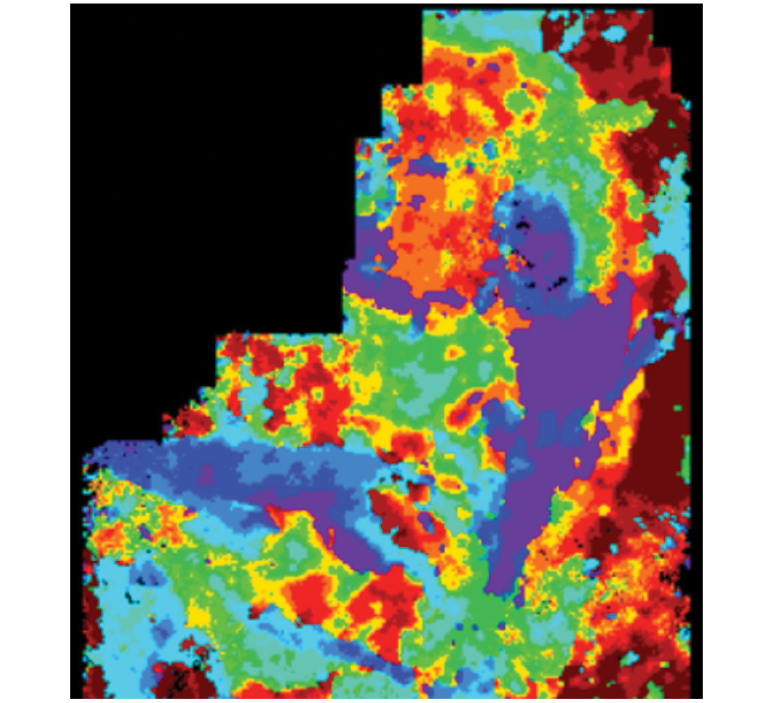
Figure 10 shows how waveform identification was used for identification of anomalies. Notice that the anomalies seen in purple are close to what was found on the AVO attribute slices shown in Figure 6.

Texture attributes

More recently the idea of studying seismic ‘textures’ has been revived. While the term was earlier applied to seismic sections to pick out zones of common signal character (Love and Simaan, 1984), studies are now underway to use statistical measures to classify textures using gray-level co-occurrence matrices (Vinther et al., 1995; Vinther, 1997; Whitehead et al., 1999; West et al., 2002; Gao, 2003, 2004). Some of the statistical measures used are energy (denoting textural homogeneity), entropy (measuring predictability from one texel or voxel to another), contrast (emphasizing the difference in amplitude of neighboring voxels) and homogeneity (highlighting the overall smoothness of the amplitude). Energy, entropy and homogeneity have been found to be the most effective in characterizing seismic data.

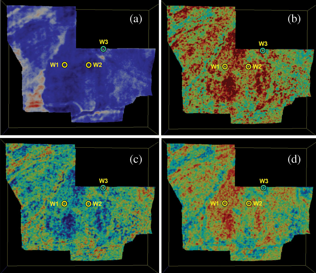
Figure 11a shows a strat-slice display from a 3D seismic volume at the reservoir level where wells W1 and W2 are producing from the same Lower Cretaceous glauconitic gas sand (Chopra and Alexeev, 2005). However, there is no indication of this on the strat-slice. Texture attribute displays comprising the energy, entropy and the homogeneity are shown in Figure 11b to d respectively. Notice the energy attribute indicates high-energy values for the producing formation for wells W1 and W2. These high values of energy are also associated with low entropy and high homogeneity, a typical combination that is expected for fluvial deposits (Gao, 2003).

Curvature

With the wide availability of 3D seismic and a renewed interest in fractures, we have seen a rapid acceleration in the use of curvature maps. The structural geology relationship between curvature and fractures is well established (Lisle, 1994) though the exact relationship between open fractures, paleo structure, and present- day stress is not yet clearly understood. Roberts (2001), Hart et al. (2002), Sigismondi and Soldo (2003), Massafero et al. (2003) and others have used seismic measures of reflector curvature to map subtle features and predict fractures. Curvature (a three dimensional property of a quadratic surface that quantifies the degree to which the surface deviates from being planar) attribute analysis of surfaces helps to remove the effects of regional dip and emphasizing small-scale features that might be associated with primary depositional features or small-scale faults.

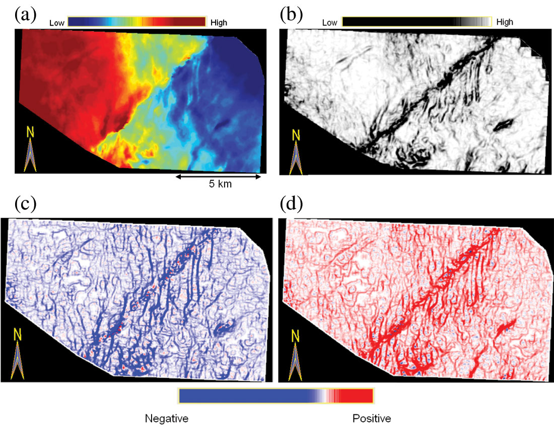
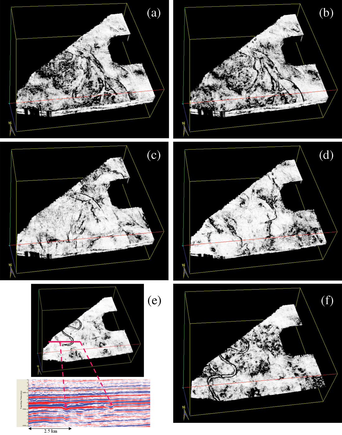
Figure 12a shows a comparison of a time surface from a 3D seismic volume in northwest Alberta. The time surface indicates a prominent fault crossing a couple of narrow vertical channels. On the equivalent coherence display (Figure 12b) the main fault and boundaries of some of the channels can be seen clearly. The most negative curvature display (Figure 12c) indicates the base of the narrow channels and how the fault intersects them is evident. The most-positive curvature images the edges of the channels clearly. Notice the crisp definition of one of the channels shown with blue arrows on the most-positive curvature (Figure 12d) and the base of the channel imaged clearly on the most-negative curvature (red arrows in Figure 12c).

A similar comparison is shown in Figure 13 where a meandering channel is the only prominent feature seen to the left of the time surface (Figure 13a). The equivalent coherence display (Figure 13b) shows a crisper definition for the channel and a couple of other features indicated with arrows. The most-negative curvature ( Figure 13c) shows the base of the channels seen in Figure 13a, but the lower main channel boundary is seen in a different direction (magenta arrow). In fact, there is another channel seen to the southwest of the image. The edges of the channels are seen clearly in Figure 13d.

Examples of present-day workflows

(1) Attributes used to generate sand probability volumes:

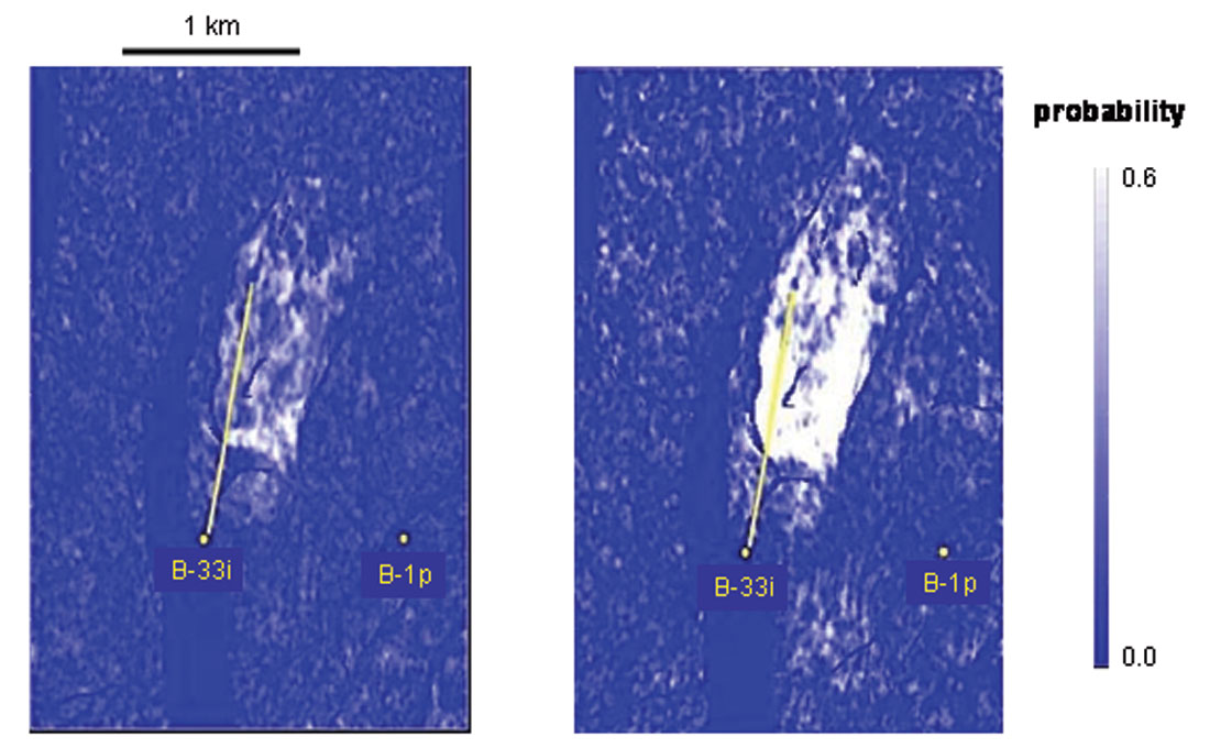
When attributes are tied to the available well control, they can be correlated to petrophysical properties, and this helps the interpreter to identify and associate high correlations with specific properties. For example, Figure 14 shows how attributes from prestack inversion of a high-resolution seismic dataset allowed mapping of sand bodies in a geologically complex area. A key step in the workflow was the petro-elastic analysis of well data that demonstrated that seismic attributes derived from prestack seismic inversion could discriminate between sands and shales.

A multi-attribute classification approach, incorporating neural network training techniques, was used to generate sand probability volumes derived from P-wave and S-wave impedances estimated using AVO inversion. The study demonstrated that high- resolution seismic data coupled with targeted inversion can increase confidence and reduce uncertainty.

A crucial problem in any multi-attribute analysis is the selection and the number of seismic attributes to be used. Kalkomey (1997) showed that the probability of observing a spurious correlation increases as the number of control points decreases and also if the number of seismic attributes being used increases. A way out of such a situation is to withhold a percentage of the data during the training step and then later to use this hidden data to validate the predictions (Schuelke and Quirein, 1998).

(2) Time-lapse analysis:

(a) Seismic attributes are being used effectively for time-lapse data analysis (4-D). Time-lapse data analysis permits interpretation of fluid saturation and pressure changes, and helps understanding of reservoir dynamics and the performance of existing wells.

Figure 15 shows an example from east of Schiehallion field West of the Shetlands (Parr and Marsh, 2000). The pre- production surveys in 1993 in (a) and 1996 in (b) show a high degree of similarity, but the 4-D survey (in (c)) shows large changes around producers and injectors. The poor production rates and low bottom hole-flowing pressures led to the conclusion that well C was located in a compartment that is poorly connected to injection support. The areal extent of this compartment could be picked by the amplitude increase seen on 4-D image and interpreted due to gas liberated from solution. This area is consistent with predictions from material-balance calculations.

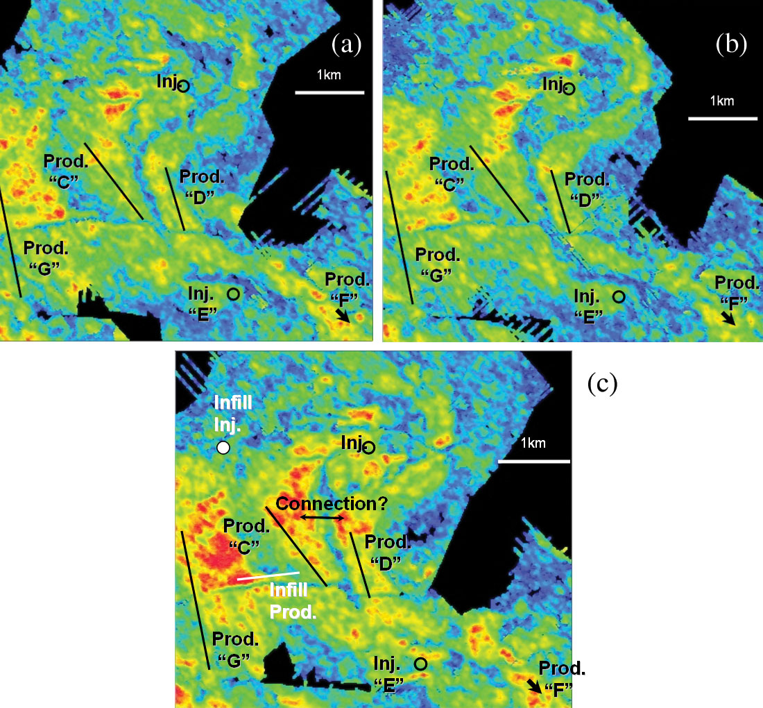
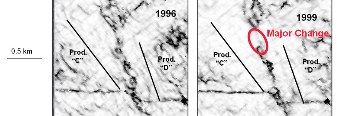
Figure 15c from the 1999 survey suggested the possibility of a connection (marked by an arrow) between producers C and D. The existence of such a connection was also suspected from the material-balance analysis. Figure 16 shows a coherence display at the required level and depicts the expected connection (marked by a circle). While a plausible explanation for this is not known, it is postulated that the attributes on 4-D seismic provide a clue that a transmissibility barrier may have been broken between the injector and producer.

(b) Reservoir based seismic attributes are being used to help delineate anomalous areas of a reservoir, where changes from time-lapse are evident (Galikeev and Davis, 2005). As for example, reservoir condition due to CO₂ injection could be detected. They generate attributes that represent reservoir heterogeneity by computing short time window seismic attributes parallel to the reservoir. Such an analysis in short temporal windows ensures that attribute carries an overprint of geology (Partyka et al., 1999).

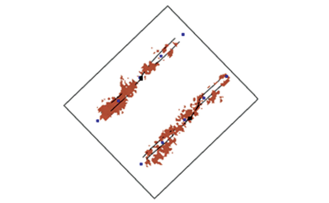
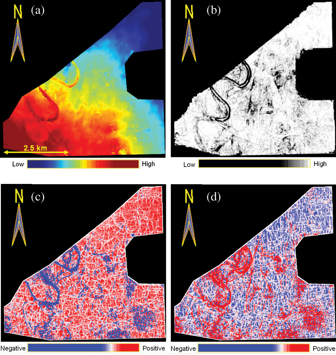
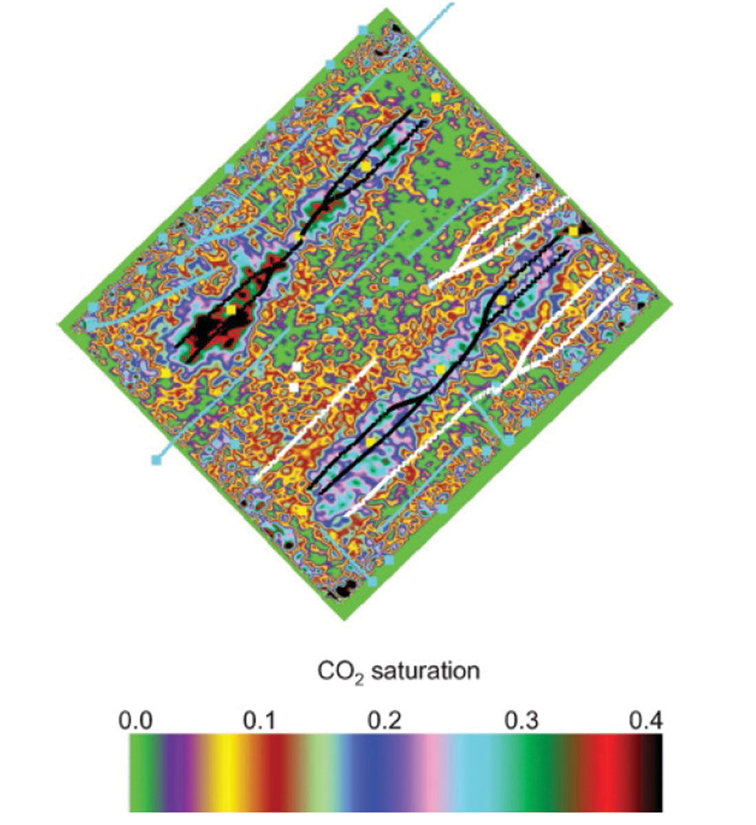
Figure 17 shows the dynamic changes within the Weyburn reservoir (Canada), due to the increased CO₂ saturation. This was done by computing the inverted impedance model of the reservoir on the differenced volume of the baseline (2000) and second monitor (2002) surveys. Figure 18 is a computed CO₂ saturation map, where the values do not represent absolute CO₂ saturation, but rather an estimation of part porosity occupied by CO₂ after irreducible water and oil were taken into account.

(c) 4-D seismic attributes together with 4-D rock and fluid analysis and incorporation of production engineering information, have been used for pressure-saturation inversion for time-lapse seismic data producing quantitative estimates of reservoir pressure and saturation changes. Application of such an analysis to the Cook reservoir of the Gulfaks field, offshore Norway (Lumley et al., 2003), shows that a strong pressure anomaly can be estimated in the vicinity of a horizontal water injector, along with a strong water saturation anomaly drawing towards a nearby producing well (Figure 19). This is in addition to strong evidence of east-west fault block compartmentalization at the time of the seismic survey.

(3) Attributes for detection of gas zones below regional velocity inversion:

Evaluation of gas distribution in the fluid system in the Wind River Basin where there are anomalously pressured gas accumulations is a challenge. Using the available logs and seismic data, the regional velocity inversion surface has been mapped in this area (Surdam et al., 2004b), which is the pressure surface separating the anomalously pressured rocks below from the normally pressured rocks above. Seismic attributes have been successfully used to evaluate the distribution of sandstone rich intervals within the prospective reservoir units. The Frenchie Draw gas field in the Wind River Basin is an example of an area where detecting and delineating gas zones below the regional velocity inversion surface is difficult. The stratigraphic interval of interest is the Upper Cretaceous-Paleocene Fort Union/Lance lenticular fluvial sandstone formations on a north plunging structural nose. The gas distribution pattern in the formations has been found to be complex, and so the exploitation proved to be risky. Surdam (2004a) has demonstrated that a good correlation exists between seismic frequency and gamma ray logs (lithology) in the lower Fort Union/Lance stratigraphic interval. The frequency attribute was used to distinguish sandstone-rich intervals from shalerich intervals.

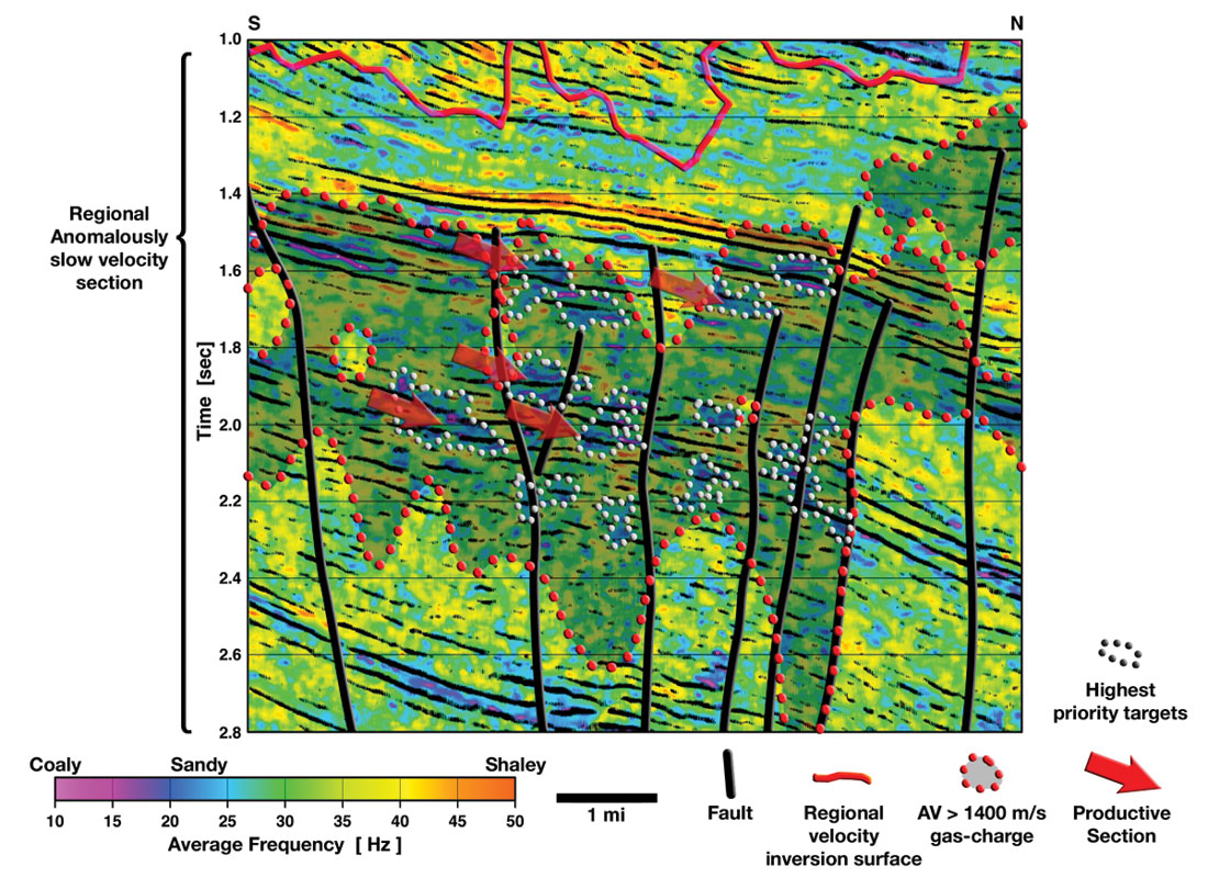
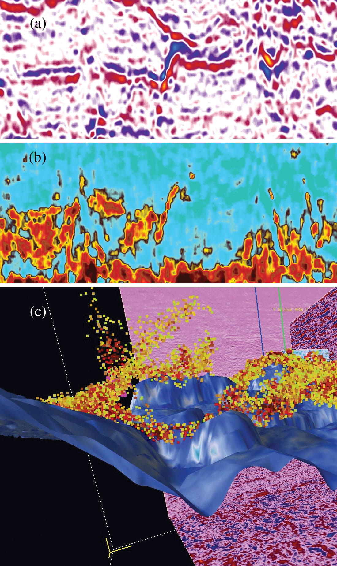
Figure 20 shows a frequency attribute section (with seismic data overlaid) covering the Fort Union/Lance stratigraphic interval intersecting the anomalously slow velocity domains (outlined by white dots). In addition to the north-plunging structural nose seen in the area, a shale rich sequence (seen in orange) is seen near the upper edge of the gas production. The important thing seen here is the lenticular distribution of the sandstone-rich intervals in blue that stand out against the shale-rich intervals in orange, yellow and green. This distributional pattern of lithologies corresponds well with the initial interpretations carried out by geoscientists who discovered the field.

The present

There are many areas in the attribute world where active development is underway and we mention here some of the prominent ones.

1. Volumetric estimates of curvature:

Cracks or small discontinuities are relatively small and fall below seismic resolution . However, the presence of open and closed cracks is closely related to reflector curvature (since tension along a surface increases with increasing curvature and therefore leads to fracture). Until now, such curvature estimates have been limited to the analysis of picked horizons, which previously may be affected by unintentional bias or picking errors introduced during interpretation. Volumetric curvature computation entails, first, the estimation of volumetric reflection dip and azimuth that represents the best single dip for each sample in the volume, followed by computation of curvature from adjacent measures of dip and azimuth. The result is a full 3D volume of curvature values at different scales of analysis (al Dossary and Marfurt, 2006).

2. 3D classifiers:

Supervised 3D classification is being used for integrating several seismic attributes into a volume of seismic facies (Sonneland et al., 1994, Carrillat et al., 2002). Some of the most successful work is in imaging by-passed pay (Xue et al., 2003) using attributes sensitive to amplitude and trace shape. Workers at deGroot-Bril, Paradigm, Rock Solid Images and many others have made progress in using geometric attributes as the basis to automatically pick seismic textures in 3D.

3. Structurally-oriented filtering:

Recently, several workers have used the volumetric estimates of dip and azimuth to improve the signal to noise ratio, yet preserve discontinuities such as faults and stratigraphic discontinuities. Hoecker and Fehmers (2002) use an anisotropic diffusion algorithm that smoothes along dip azimuth only if no discontinuity is detected. Luo et al. (2002) use a multi-window analysis technique, smoothing in that window containing the analysis point that has the smallest variance. Duncan et al. (2002) built on this latter technique, but instead of a mean filter, applied a principal component filter in the most coherent analysis window. These structurally-oriented filtering (alternatively called edge-preserving smoothing) algorithms improve not only behavior of autotrackers but also the results of coherence and other attributes sensitive to changes in reflector amplitude, waveform, and dip.

4. Volumetric estimation of Q:

The most common means of estimating Q is through sample by sample estimates of spectral ratios. Typical workflows use a smoothly varying estimate of Q to increase the spectral bandwidth at depth. Most workers have focused on intrinsic vs. effective Q, the later including effects such as geometric scattering and friendly multiples. The most promising work is done with the aid of VSPs and/or well logs. In these flows, one can interpret not only the spectral amplitude but also the spectral phase compensation necessary to improve seismic resolution.

5. Pre-stack attributes:

In addition to AVO, which measures the change in reflection amplitude and phase as a function of offset at a fixed location, we can apply attributes such as coherence and spectral decomposition to common offset volumes to better predict changes in lithology and flow barriers. While the interpretation is entirely consistent with AVO analysis, the 3D volumes tend to show discrete geologic features and the limits of hydrocarbon distribution. There is a similar relationship between amplitude vs. azimuth and geometric attributes applied to common azimuth volumes. In this latter case, we often find faults and fractures better illuminated at those acquisition azimuths perpendicular to structural trends.

Gazing into the Future

Given the current data explosion both of large regional 3D surveys, but also of new time-lapse and multicomponent surveys, we envision an increasingly rapid evolution of seismic attributes and computer-aided interpretation technology. Some of the clear signs on the horizon are as follows:

1. We expect continued development of texture attributes that can quantify or enhance features used in seismic stratigraphy and seismic geomorphology leading to computer-aided 3D seismic stratigraphy. One of the major challenges is that due to tectonic deformation and sedimentary compaction, such patterns may be arbitrarily rotated from their original position.

2. We expect enhanced emphasis will be placed on time-lapse applications for delineation of flow-barriers, so that reservoir simulation provides more realistic estimates and information regarding the dynamic behavior of reservoirs.

3. We expect continued advances in 3D visualization and multi-attribute analysis including clustering, geostatistics, and neural networks to alleviate the problems interpreters face due to an overwhelming number of attributes.

Conclusions

A seismic attribute is a quantitative measure of a seismic characteristic of interest. Good seismic attributes and attribute analysis tools mimic a good interpreter. Over the past decades, we have witnessed attribute developments track breakthroughs in seismic acquisition and reflector mapping, fault identification, bright spot identification, frequency loss, thin bed tuning, seismic stratigraphy, and geomorphology. More recently, interpreters have used crossplotting to identify clusters of attributes that are associated with either stratigraphic or hydrocarbon anomalies. Once again, the attribute community has worked hard to first duplicate such human-driven clustering through the use of self-organized maps, geostatistics, and neural nets, and then to extend this capability beyond the three dimensions easily visualized by interpreters. Tentative steps have been made towards computer- assisted seismic stratigraphy analysis, whereby an interpreter trains the computer on a suite of structural or depositional patterns and asks the computer to find others like them. Progress has been made in automated fault tracking, though currently the technology requires an expert user. In the not too distant future, we can envision an interpreter seeding a channel on a time slice after which the computer paints it in 3D. Although it may take decades, we expect computers will eventually be able to duplicate all the repetitive processes performed by an interpreter. In contrast we do not expect them ever to replicate the creative interpreter imagining depositional environments, structural evolution, diagenetic alteration, and fluid migration. The human interpreter is here to stay, but may be offshored in the future.

Acknowledgements

This paper is an off-shoot of a more comprehensive review paper published in Geophysics (Chopra and Marfurt, 2005). We wish to thank many individuals for the help we received in the writing of that paper, amongst which the following names would figure prominently: Nigel Anstey, Tury Taner, Jamie Robertson, Alistar Brown, Roy Lindseth, Brian Russell, Roy White, Les Hatton, Bob Sheriff, Sven Treitel, Bee Bednar, Jerry Schuster and Art Barnes.

Finally, we thank Ronald Parr for Figures 14 and 15, Tom Davis for Figures 16 and 17, Mark Meadows for Figure 19, and Ron Surdam for Figure 20.

We have tried to cover almost all the prominent developments in this vast field of seismic attributes. However, in spite of our best efforts, it is likely we may have missed out on some. Hence any errors or omissions were unintentional and solely our responsibility.

One of the authors’ (S.C.) expresses his appreciation to Arcis Corporation, Calgary for permission to use some of the data examples and publish this paper.