Reservoir vs. Seal Pressure Gradients: Perception and Pitfalls – Based on Case Histories from the Gulf of Mexico

There is confusion about the calculation of pore pressure gradient in permeable beds (reservoirs) versus very low permeable beds (seals) especially in the geopressured section.

The four subsurface geopressure zones, introduced in this paper, explain the fundamentals of pressure measurements and predictions of reservoirs vs. seals. Reservoir and seal pressure gradients in each of these zones behave differently. The change of the gradient slope is contingent on the formation's fluid density and the vertical subsurface compartmentalization. Exploration risk and drilling challenges are greatly impacted by the subsurface geopressure gradients changeability.

Geoscientists are inclined to use pressure values in psi and kPa. On the other hand, drilling engineers prefer to calculate subsurface pressure values expressed in pound per gallon mud weight equivalent (ppg mwe). Therefore, the industry adopted a hybrid pressure-depth plot combining the pressure in psi and ppg mwe at the same display. As a consequence, standard gradient conversion factors of 1/0.052 emerged as a mathematical transformation factor from psi/ft to ppgmwe; and 0.852 from kPa/M to ppgmwe. These conversion factors can be acceptably used in the seals; however it is erroneously applied in the reservoirs.

Equating the subsurface geopressured entrapped fluid in the reservoir to the man made changeable mud pressure leads to incorrect calibration of pore pressure prediction models, as well as creating fictitious pressure regressions in most of the reservoirs. Moreover, this erroneous hybrid depth vs. psi – ppg combined plot gave birth to a new phenomenon identified as the Centroid.

Subsurface geopressure compartments

Pore pressure gradient in the subsurface is dictated by stress, permeability and, most importantly, compartmentalization. Subsurface compartments are mainly formed due to changes in lithology, sedimentation rate and structural patterns.

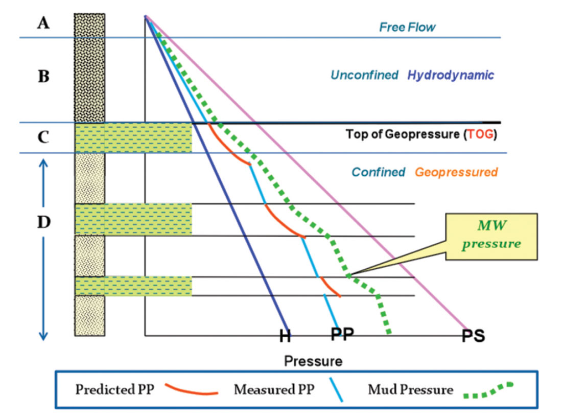
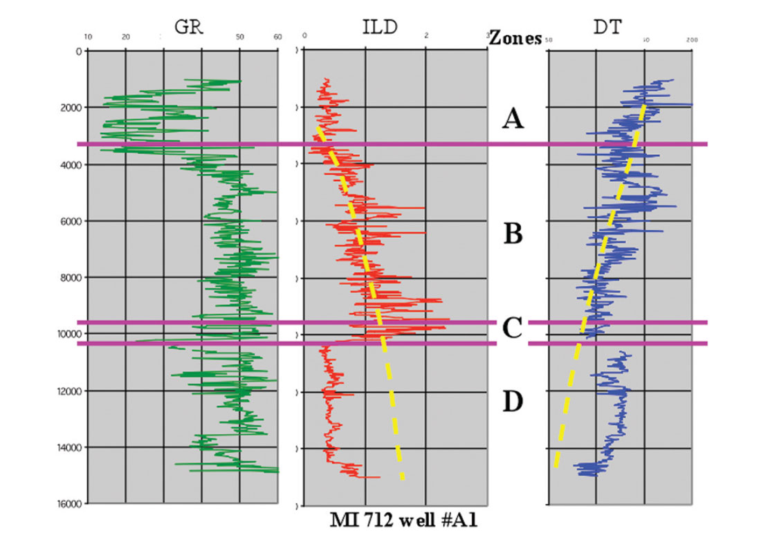
The vertical generic pore pressure profile in the subsurface can be, in most cases, divided into four zones. This finding is based on integration of a large data base of pressure (Figure 1) and petrophysical (Figure 2) measurements from the Gulf of Mexico area:

A– The very shallow free flow section (A) is usually in communication with the seafloor in offshore and groundwater onshore. The thickness of this thin zone relies on the input sediments lithology from the deposition feeders system. The fluctuation in sea level and groundwater flows impacts the hydrologic behavior of this zone in offshore and onshore respectively. The top of this zone is at the mud line (sea bed) in offshore and is at the ground-water table in onshore. The base of this zone is defined at a depth where the process of dewatering starts (top of zone B); where the low permeable sediments and overburden stress reach the disequilibrium phase.

The encroachment of brackish and fresh water in this zone sometimes leads to higher well log resistivity measurements (Figure 2).

Offshore, the pressure of the reservoirs and seals of these upper unconsolidated sediments has the same gradient (+/- 0.465 psi/ft in GoM) and is a function of depth and sea water density. On the other hand, onshore, where topography has a great impact on the hydrology of this zone, lateral piezometric pressure gradient applies. Potentiometric surface mapping is used to calculate ground water flow and potential hydrocarbons in this zone (Dahlberg 1994).

B– Zone (B) starts where sediments begin to expel water, to the above zone A, due to depositional load (overburden). It bottoms at the top of the geopressure (C). This unconfined hydrodynamic zone forms due to the compaction disequilibrium process. This zone shows a gradual increase of pressure gradient with depth. The pore pressure in this section increases with depth (Figure 3) in both sand and shale. It ranges from hydrostatic at the top to a higher gradient value at the bottom where the process of dewatering is ceased (Shaker, 2007). The sand and shale pressures in this hydrodynamic segment are functions of depth, formation water density, viscosity, sediment permeability and the force vector of upward flow (DP). Darcy's law would apply in this zone to establish the relationship between flow and pressure gradient:

The fluid influx between beds, from deep to shallow in this segment gives the false impression of the presence of a near surface geopressured zone.

In Keathley Canyon Block 255; where BP extensively took RFT measurements from the entire well; the upward pressure gradient decreased gradually from 0.621 psi/ft to 0.520 psi/ft between depth 11,500’ and 9800’ respectively (Figure 3).

The differential flow rate (Darcy’s flux) between the sand and clay/shale, due to permeability contrast, causes several drilling hazards. Most of these hazardous challenges occur when the drilling bit crosses from low permeable (shale/mud) layer to a sand bed below. The abrupt increase of formation water flow across beds interface leads to a strong mud cut and possibly resulted in flow – kill – loss of circulation cyclical event. This phenomenon is known in some of the deepwater exploration areas as shallow water flows (SWF).

In this zone the petrophysical properties (resistivity, velocity, and density) exhibit a gradual change with depth that corresponds with the porosity reduction due to compaction increase. The slopes on these well logs measurements (Figure 2) are referred to, by the pore pressure prediction analysts, as the Normal Compaction Trend (NCT). The shale shows an exponential NCT slope (Figure 2), whereas sand exhibits linear trend (Figure 3).

C– The transition zone (C) sets between the hydrodynamic system (B) and the confined geopressure system (D) and represents the top seal of the entire section below. It represents the top cap where fluid is not capable of escape. This section, in general, is built of a regional condensed section of high stand depositional stratigraphic sequence i.e. Cibicides opima shale in offshore Texas. The thickness of this zone can range from tens to hundreds feet.

The pressure gradient in this relatively short interval significantly increases. This pressure transgression is contingent on the seal age, thickness and lithology. It is noticed that during drilling of older sediments mud weight needs to be raised three pounds to penetrate this zone i.e. Gulf Coast and shallow offshore shelf. However, in younger sediments and deep water wells, mud weight is subtly raised between one and two pounds.

This zone represents a distinct pivot point for the petrophysical properties’ measurements to change values (Figure 2). Velocity, resistivity, and density decreases, whereas, DT, conductivity and porosity increases crossing this zone.

Usually, this zone is identified in geopressure practice as the top of geopressure (TOG) or the fluid retention depth (FRD). This relatively under-evaluated zone represents the boundary between the static confined sealed zone (D) below and the dynamically breached zones (B /A) above.

This zone signifies the most profitable cut off drilling depth for finding hydrocarbon without setting an intermediate casing seat. Moreover, the hydrocarbon optimum trapping mechanism is favorable just above this zone where hydrocarbon migration takes place from the geopressured (D) to the hydrodynamic (B) section.

D– The reservoirs and seals in this static geopressured zone (D) show distinctly different pressure gradients, however, they form an overall cascade-shaped progressive profile (Figure 1). Reservoir pressure shows a static linear gradient contingent on the fluid’s density (water, brines, oil, and gas) in the pore spaces. The pore pressure in reservoirs can be calculated as follow:

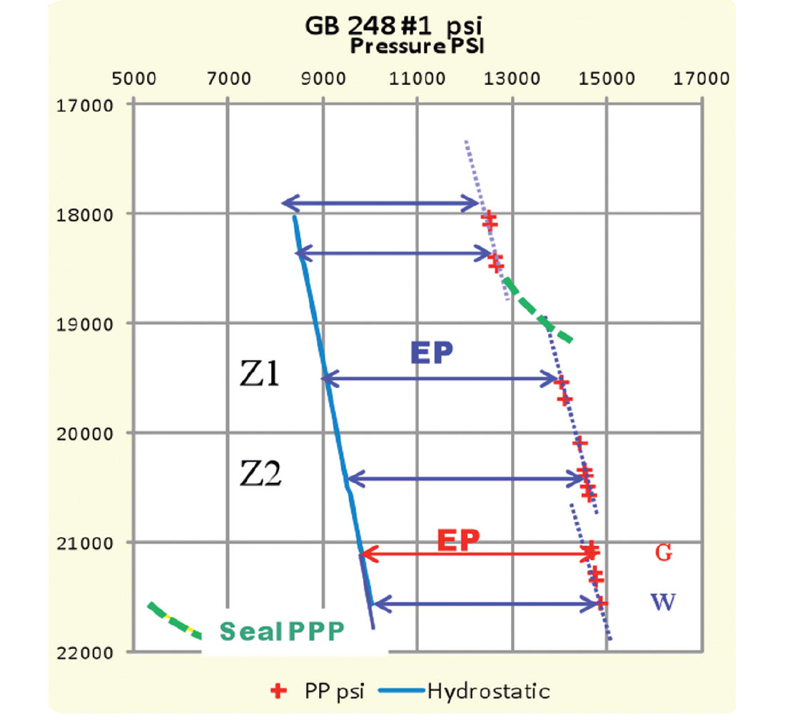
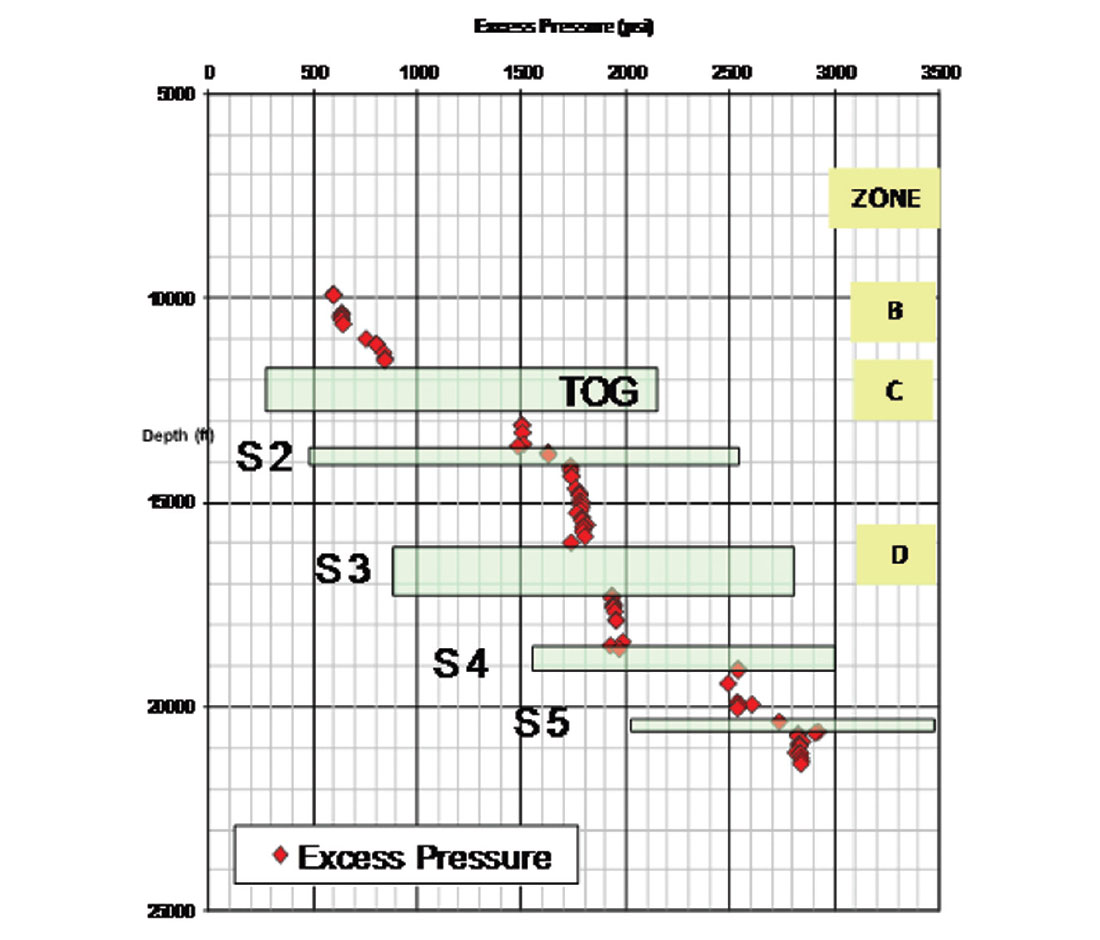
The excess pressure (EP) in a reservoir is the difference between the reservoir pressure and the regional hydrostatic pressure at Z depth (Shaker 2001):

This EP window should be constant in a single wet reservoir (Figure 4). Therefore:

In Garden Banks 248 well #1, note the presence of three compartments and each wet reservoir compartment carries the same EP. However, the lower pay zone between 21,000’and 21,700’ shows a larger EP at the hydrocarbon bearing zone than the wet sand below due to the steep gas gradient.

To predict pore pressure at depth Z2 in a virgin reservoir where pressure is known at Z1 (Figure 4):

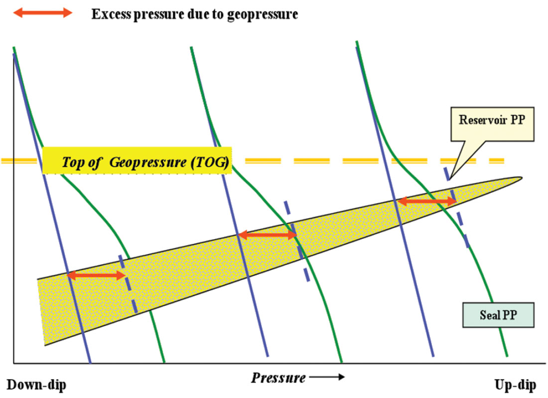
The sealing capacity (SC) represents the pressure shift between the consecutive compartments (Figure 5). The successive subsurface compartments pressure (envelopes) should bear the same fluid formation gradient, as long as the paleo-formation water salinity stays in the same proximity. The shift from one pressure envelope to a deeper one across the seal defines the sealing capacity of the inter-bedded seals (Shaker, 2001).

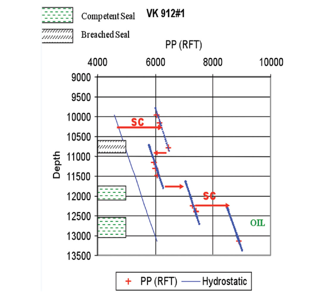
Competent seal is represented by a positive shift, whereas negative shift (Figures 4 and 5) reflects breach due to a structural failure (fault, salt interface, unconformity .etc). On the other hand, the alignment of pressure measurements of several compartments indicates communication (Figure 11 and 12).

Virgin reservoir (in the absence of hydrocarbons) usually exhibits the hydrostatic gradient of the formation fluid (0.46 psi/ft in GOM) and progresses in a cascade fashion with depth crossing the intercalated seals (Figures 1, 4 and 5).

Wire-line tools; such as repeated formation tester (RFT), modular dynamic tester (MDT) etc; measure pressure in permeable beds at specific depth. Noteworthy, shut in pressure (SIP) represents the formation pressure at the well head of the reservoirs in the uncased open-hole section.

Moreover, the reservoir bears a hydraulic head as a result of the excess pressure (Figure 6).

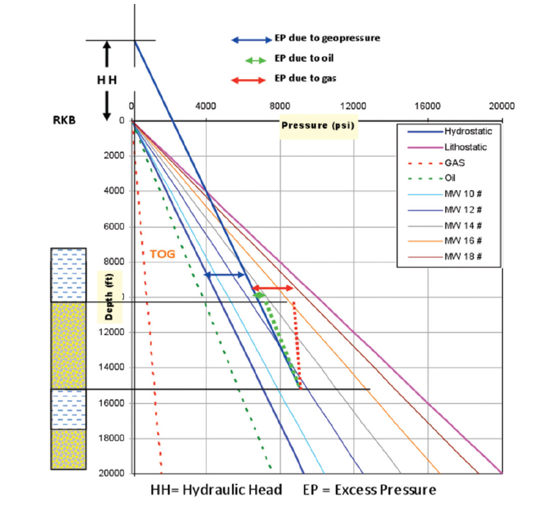
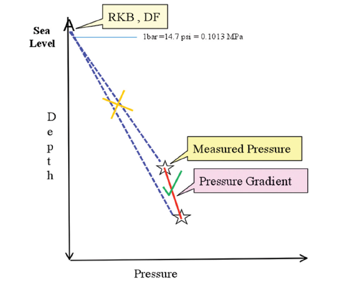
The hydraulic head (HH) is the potential height of the formation fluid (water, oil or gas ) to rise above a reference point i.e. RKB, Sea level, well head, ground level (Figure 6). The excess pressure in Zone D and the potentiometric difference on-land are the driving mechanism for generating the HH. The height of HH can be calculated:

Noteworthy formation water, oil, and gas pressure gradient follow linear trends, contingent on their density, in permeable reservoirs (Figure 6). The linear trends in multiple phase reservoirs change gradients at the interception point e.g. water/oil/gas contacts.

On the other hand, the pressure in the seals tends to follow a higher gradient (Figures 4, 8 and 10) that mimic the lithostatic stress (overburden in a relaxed tectonic system). The pressure gradient in the shale is directly impacted by changes of porosity due to burial, compaction and fluid loss. It shows exponential trends and follows the logarithmic porosity compaction trend of Athy’s 1930:

Moreover, the widely used effective stress – pore prediction transformation models in the seals (shale) are based on exponential/ power-law trends (Figures 1, 2 & 4).

The shale’s sonic-pore pressure prediction relationship is expressed as follows:

The principal stress plays an essential role in the pressure’s acceleration of the overall (seals and reservoirs) subsurface profile. The anticipated cascade-shaped progressive pressure profile sometimes changes course and shows regressive trends (Figures 4 and 5). The divergence between the pore pressure in the shale (PPP) and the sand (MPP) is a consequence of the principal stress magnitude and compartmentalization. The geological building blocks, mainly sedimentation pattern and structural lineaments, control entrapment and breaching of the formation fluids in the different subsurface compartments.

Mud pressure

The drilling mud has inherited the role of cutting removal and drilling bit lubrication during the early drilling era. Bore-hole stability became an essential mud function after exploration expanded deeper in the highly geopressured environments.

The pressure generated at the drilling bit and the bore-hole walls by the drilling mud column is variable and corresponds to the mud density (Figure 6). Mud pressure is usually measured from a fixed reference point (e.g. Kelly bushing or derrick floor). The mud pressure gradient is always linear through the casing and open hole.

In the geopressured environment, maintaining the balance between the mud pressure and reservoirs/seals pressures, during drilling, is a very intricate process. If the predicted drilling mud weight is less than the actual reservoir pressure (under-balanced), sand beds flow and mud cut and possible hard kicks take place. Moreover, the shale section becomes instable and wall caving with extensively enlarged well bore diameter can be created.

Loss of circulation, tight hole and high torque are common drilling challenges when of the predicted mud pressure is extensively higher (over-balanced) than the actual reservoir pressure. In addition, shale beds can suffer from micro-fracturing and ballooning.

Pressure gradient’s measurement

Calculating the pressure gradient in reservoirs using RFT, MDT etc. data should be calculated between, at least, two depth point records in the same compartment (Figure 7). Referencing the reservoir geopressured gradient to the subsea level (SL), Kelly bushing (RKB) and Derrick Floor (DF) causes serious mistakes in calculating the reservoir formation’s fluids gradient, density and hydrocarbon type (water, oil, and gas). On the other hand, since shale is not capable of flowing, as opposed to sand; pressure gradient in shale can be calculated from the RKB.

The shale pore pressure is predicted using seismic velocity before drilling. During and after drilling, a bundle of petrophysical wire line measurements can be used to determine the shale pressure gradients in the different seals below the top of geopressure. As we discussed previously, seals pressure gradient follow power–law forms.

Mud pressure gradient can be expressed in psi/ft, ppg (pound per gallon), kPa/M, and g/cc. The standard gradient conversion factor of 1/0.052 is used to convert mud pressure from psi/ft to ppgmwe; and 0.852 from kPa/M to ppgmwe and vice versa. The mud pressure follows linear trends with an interception point at the RKB. The slopes on the gradient lines vary contingent on the mud weight. They take a fan shape (mud fan) with its tip at RKB if plotted in psi (Figure 6 and 9) and form vertical grid lines if plotted in ppg on P-D plots (Figures 12 and 13).

Mud weight can be sampled from the mud pit (expressed in ppg) or measured (in psi) at the BHA (bottom hole assembly) which is known as ECD (equivalent circulating density).

Measured mud pressure using the RFT and MDT tools does not represent the real time values, during drilling, since this measurement takes place post drilling in a non circulating mud condition (Figure 10).

The impact of structural tilt on reservoir – seal pressures

It is known that reservoir pressure at the crest of a structural closure shows higher pressure values than the predicted shale pressure and vice versa on the prospect’s structural flanks.

As we previously discussed and justified, the pore pressure in a single geopressured compartment should bear the same excess pressure. As a result, the structural tilt should not impact the gradient or the excess pressure window in the reservoir (Figure 8). The sealed porous and permeable geopressured reservoir should follow the static hydraulic laws in a non flow system. Therefore, the fluid density is the main pressure driving mechanism in a reservoir. The vertical pressure calculations should be based on equations 1, 2, 3 and 4 in this article.

Zhang 2011, stated “The pressures in a hydraulically connected formation can be calculated based on the difference in the heights of fluid columns, i.e.:

where p1 is the formation fluid pressure at depth Z1; p2 is the formation fluid pressure at depth of Z2; ρf is the in-situ fluid density; g is the acceleration of gravity.

On the contrary, shale pressure is a function of the principal stress magnitude (Terzaghi 1943). In the presence of larger overburden on the structural low, shale seems to have a higher pressure. Conversely, on the structural crest, where thinner overburden exists, shale bears less pressure.

On the other hand, reservoir has the same pressure gradient and constant excess pressure within the entire tilted exploration structural closure i.e. sealed reservoir. Therefore, it appears that the encased sand’s pressure is relatively lesser than shale pressure on the structural low and larger than shale on the crest and structural high (Figure 8).

Dickinson (1953) in one of his conclusions showed that pressure gradient, in a tilted reservoir, decreases with increasing of depth. He was calculating the pressure gradient in reference to subsea depth (SL). His conclusion that pressure gradient decreases with depth in a structurally tilted reservoir was an unintended misleading calculation. This is one of the common pitfalls in geopressure calculations (Figure 7).

Traugott and Heppard (1997) applied the hybrid depth-psi / ppg plot to convert the pressure in the reservoir from psi to ppgmwe. This led to the belief that there is a midpoint on the structure (Centroid) where the pore pressure in the reservoir and seal have the same value. Their hypothesis states that sand pressure (in ppgmwe) increases above the Centroid point, and, decreases below this midpoint. This gives an artificial impression of pressure regression on most of the reservoirs. This is another common pitfall of using the standard conversion factor (SCA) in converting pressure from psi to ppg mwe in geopressured reservoirs.

The standard conversion factor is derived as follows

From lb/gal to psi/ft ... 12in³/231 in³=0.052 and vice versa from psi/ft to lb/gal …. 1/0.052=19.2. The SCA is based on KB as the reference point.

This mathematically driven SCF is embedded in most of the pore pressure prediction software. Bruce and Bowers (2002) stated in the pore pressure special section of the TLE “Without question, expressing the pore pressure in unit of density is scientifically incorrect.”

The display on figure 9 shows in depth the details of a reservoir pp gradient’s miscalculation when the hybrid psi / ppg plot is applied. The PP in ppg, as shown from the interception of the reservoir PP in psi with the mud fan lines, exhibits decreasing values with increasing depth. The reservoir pressure trend line intercepts higher MW equivalent of 16# at depth 9,000’ and intercepts a MW equivalent of 13# at depth 17,000’.

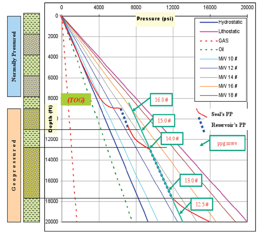
The argument here is why the actual reservoir pressure in psi increases with depth and conversely, decreases with depth in ppgmwe? This is because the SCF of 0.052 and 0.852 should not be applied in converting pressure from psi to ppgmwe in geopressured reservoirs. However, it is applicable in converting the geopressured shale and normally pressured sediments gradients from psi to ppgmw due to the lack of hydraulic head.

Therefore, the fictitious pressure regression that appears on most of the converted RFT, MDT data from psi to ppgmwe is not representing realistic physical data. This results in misleading pore pressure models calibration and possibly leads to fatal consequences (blowouts and hard kicks) during drilling operations, especially in deep water.

Shaker, (2003), discussed the technique of rectifying this controversial conversion factor (SCF).

Geological compartmentalization and hydraulic head corrections are the foundation of this new calculation model.

Case Histories

The subsurface four compartments:

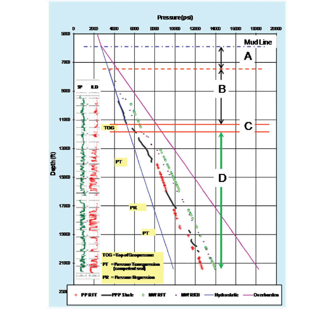
They are well displayed in KC 255 #1 due to the availability of extensive RFT’s and petrophysical measurements (Figure 10). This figure exhibits:

• The four subsurface compartments.
• The incremental pressure gradient increases in Zone B due to dewatering as result of compaction disequilibrium (Figures 3 &10).
• The PP surge of 1000 psi penetrating the 300’ thick top of geopressure (TOG) of Zone C.
• The linear hydrostatic pressure gradients in all reservoirs (PP RFT) and the exponential trend in all seals (PPP shale) in the geopressured Zone D.
• Pressure transgressions (PT) and regressions (PR) due to geological setting.
• The disparity between the MW RFT measurement (post drilling) and the real time MW RKB.

Excess pressure as sealing capacity indicator:

Using the calculated excess pressure (EP) sheds light on the seals trapping competency. Calculating (Equations 2 & 4) and plotting the EP vs. depth for the same well is an excellent sealing assessment method. The graph straightforwardly points to the competent seals and breach reservoirs in the bore-hole trajectory. Figure 11 shows:

• The TOG can trap a hydrocarbon column (if present) with EP of 700 psi in the reservoir below
• The sealing capacity is not contingent on the seal thickness. S3 is much thicker than S4, however the reservoir below S3 is breached and S4 seal can hold 500 psi. Subsurface structural failure is likely to create a breach between reservoirs rather than fracturing the top seal.

Pressure gradient reversal due to the SCF:

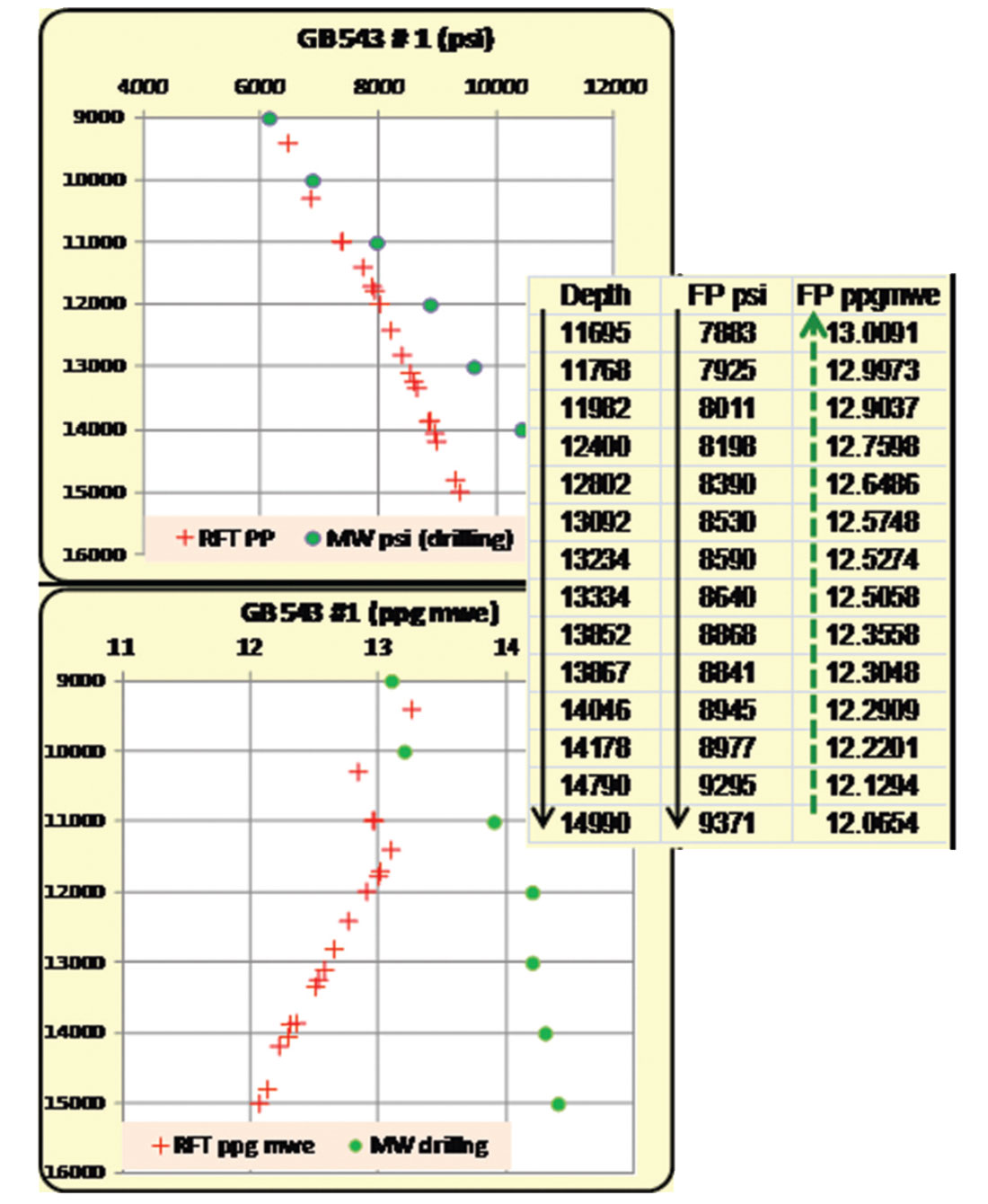
Converting the reservoirs PP from psi to ppg mwe using SCF is one of the serious pitfalls in geopressured reservoir calculations. Figure 12 shows an example of 3,500’thick (11,500’- 15,000’) geopressured reservoir where pressure was measured in psi and consequently converted to ppg mwe (table in Figure 12). Figure 12 exhibits:

• Hydraulic head can be calculated (Equation #5) at any depth (table in Figure 12). For example at depth 14,790’ H.H. is +5,200’ RKB.
• The drilling mud pressure in psi increases with depth to exert the gradually increasing reservoir pressure with depth (upper panel on figure 12). This is the factual and realistic values.
• On the other hand, plotting the RFT (FP) values in ppg mwe using the SCF (lower panel on figure 12) shows a negative declining (reversal) trend (from 13# to 12#) while the actual drilling mud weight shows a positive increase trend (from.13.5 # to 14.5#). This is physically unrealistic for drilling operations.

Pore pressure modeling calibration:

Calibration of the pore pressure prediction model in the shale (seals) can be done by incorporating the measured pressure in the sands (reservoirs). This can be successfully performed if the transformation model is totally built in psi measurement. Calibration of the PPP shale model in figure 10 was successfully done using the reservoir RFT’s integrated with the mud logs. The calibration model used E 0.35 and one contiguous normal compaction trend on the entire well.

On the other hand, if the prediction model is designed in ppg mwe, the results would be confusing and can lead to unsuccessful forcasting results. Predicting the pore pressure in the same KC 255 #1 using the SCF proves the difficulty and uncertainty of forecasting the model variables and exponents. Several iterations were processed using different exponents and the final results were not satisfactory.

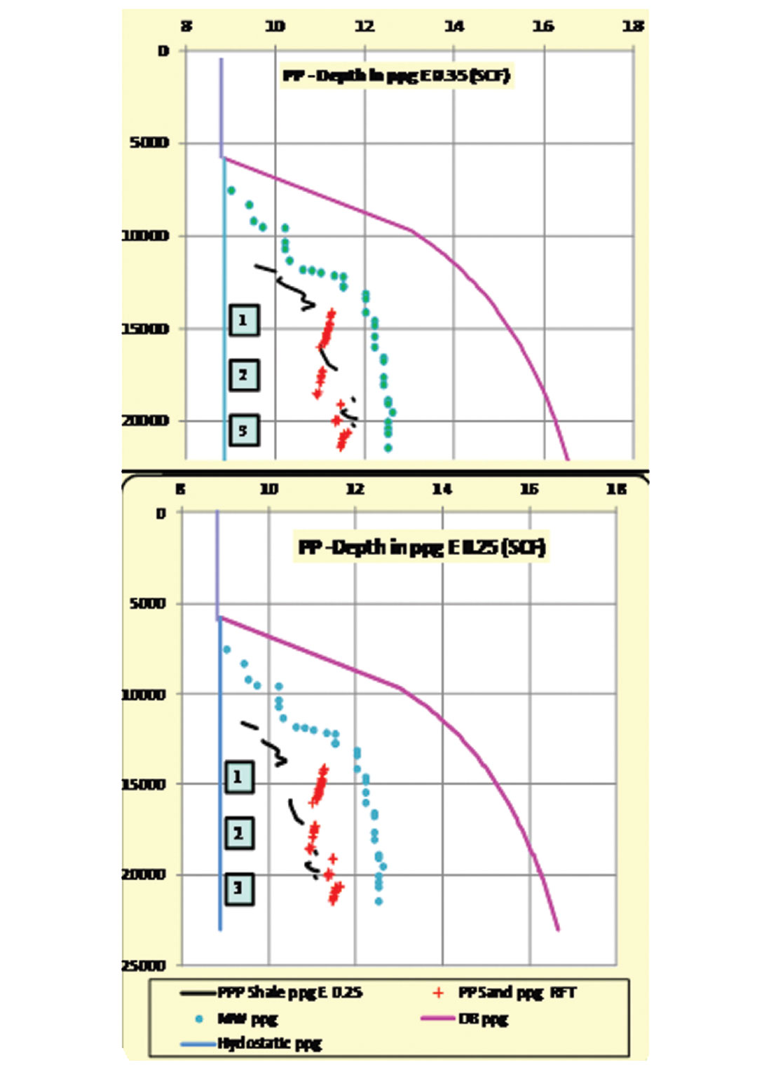
Figure 13 shows two prediction models in ppg mwe using two different exponents. It is noticed:

• In the upper panel of the figure, there is an agreement between the ppp shale and the pp sand at compartment #1 by applying the exponent E 0.35. However, compartments #2 & #3 are in disagreement with the prediction result.
• By applying the exponent E 0.25, there is an agreement between the ppp Shale ppg and the pp Sand ppg RFT at compartment # 2 and complete disagreement in compartment #1

To overcome the mismatching between the measured and predicted pressure values, breaking the Normal Compaction Trend to several segments became a calibration practice. This is another pitfall in pore pressure modeling calibration

• All the reservoirs in both models show negative slopes.
• In both models can you envision Centroid point in each reservoir?

Summary and recommendations

1. Sediments, stress and fluids are the main components of forming the subsurface geopressure four zones.
2. Pore pressure (PP) in reservoirs bears linear gradient trend contingent on the formation fluid density.
3. Predicted shale pressure follow power-law forms.
4. The shallow water flow in deep water can be attributed to the differential hydrodynamic fluid influx in zone B rather than, the presence of a very shallow geopressured zone.
5. Pressure gradient in a reservoir should be calculated between at least two measured points in the same compartment.
6. The excess pressure in the geopressured Zone (D) stays constant in the same reservoir except in pay zones.
7. The shale sealing capacity is represented and can be calculated from the pressure shift between two consecutive reservoirs.
8. Converting the reservoir pressure from psi to ppgmwe using the standard conversion factor leads to erroneous pressure profile in the geopressured (Zone D) section. However, the SCF can be used successfully in shale and Zones A & B.
9. The fictitious regression and the Centroid phenomenon are the result of using the standard mathematical conversion factor derived from the hybrid psi-ppg vs. depth plot.

Based on this study and the findings in this paper, we recommend:

1. Pore pressure gradient in geopressured reservoirs should not be calculated from reference point (RKB, DF, and SL.).
2. Using the hybrid psi-ppg mwe vs. depth plot to exhibit the PP in reservoirs lead to erroneous calculations.
3. Geopressure modeling calibration, using measured pp, should be done in psi-depth modeling format rather than ppg-depth one.
4. Breaking the Normal Compaction Trend for the purpose of fitting the ppg mwe – depth model can exacerbate the calibration problem.