Reservoir characterization by combining time-lapse seismic analysis with reservoir simulation

Summary

This study integrates time lapse seismic methods with reservoir simulation to image a steam front and by-passed oil at the Pikes Peak heavy oil field in Saskatchewan, Canada. Two seismic 2D surveys, acquired in 1991 and 2000, respectively, had been reprocessed to preserve amplitudes. Cyclical steam stimulation (CSS) of the reservoir started in 1981 and continues to the present. A flow simulation model was constructed for the region around the seismic profile. The simulator was run from the start of production in 1981 until 2000. The porosity, saturation, pressure and temperature of the reservoir zone were extracted from the flow simulation outputs for the early-production condition in 1991 and for 2000, almost 10 years later. The seismic response of the reservoir was computed using a rock physics procedure and seismic forward modelling. Comparing the seismic difference results of 1991 and 2000 and reservoir simulation outputs indicated that the gas saturation changes caused the largest change in the simulated seismic response. Seismic difference sections showed that thick zones of gas saturation caused greater time delays in sub-reservoir reflections due to the lower velocity within the reservoir zone. Thin zones of gas caused reflection amplitude differences but little time delay differences. Temperature and pressure were also correlated with seismic changes but not as quantitively as the gas saturation. The simulated seismic response difference section was compared to the measured seismic response difference section. These two difference sections are very close in characteristics although the reservoir simulation model could be adjusted in the future to make the match even better. The results indicate that the present reservoir model is reasonably good at describing the reservoir.

Introduction

Knowledge of the spatial variation of reservoir parameters such as porosity, pore-fluid content, permeability, pressure, and temperature are critical in order to evaluate accurately the total volume of recoverable hydrocarbon reserves in place and to predict fluid flow in the reservoir. Reservoir simulation is often used to help understand the changes in reservoir conditions with the stages of production. Reservoir simulation is based on models that are created from well information, seismic data and geologic maps. The results around wells are controlled by engineering data but the results between or beyond wells cannot be verified by engineering data. Seismic surveys can be used to interpolate or extrapolate reservoir information between or beyond wells. Through rock physics equations, seismic properties such as velocity and density can be estimated from the output of reservoir simulation for use in seismic modelling. Synthetic seismic sections can be created and compared with seismic field data. By analyzing the differences between the synthetic seismic sections based on the reservoir simulation and the real seismic sections, we can update the reservoir model, locate the remaining oil and trace steam fronts. There is a recognized need to combine the skills of geoscientists and engineers to build optimized reservoir models that incorporate all available engineering, geological and geophysical data. In some early research works seismic models were constructed using reservoir simulation output for primary depletion (Lumley, 1995). There are also some published seismic modelling works and simplified reservoir simulation work on steam based recovery reservoirs (Eastwood et al., 1994; Jenkins et al., 1997; Biondi et al., 1998). There is only one published example which deals with Cyclic Steam Stimulation (CSS) but the reservoir simulation results were not converted for use in seismic modelling (Eastwood et al., 1994).

Knowledge of the spatial variation of reservoir parameters such as porosity, pore-fluid content, permeability, pressure, and temperature are critical in order to evaluate accurately the total volume of recoverable hydrocarbon reserves in place and to predict fluid flow in the reservoir. Reservoir simulation is often used to help understand the changes in reservoir conditions with the stages of production. Reservoir simulation is based on models that are created from well information, seismic data and geologic maps. The results around wells are controlled by engineering data but the results between or beyond wells cannot be verified by engineering data. Seismic surveys can be used to interpolate or extrapolate reservoir information between or beyond wells. Through rock physics equations, seismic properties such as velocity and density can be estimated from the output of reservoir simulation for use in seismic modelling. Synthetic seismic sections can be created and compared with seismic field data. By analyzing the differences between the synthetic seismic sections based on the reservoir simulation and the real seismic sections, we can update the reservoir model, locate the remaining oil and trace steam fronts. There is a recognized need to combine the skills of geoscientists and engineers to build optimized reservoir models that incorporate all available engineering, geological and geophysical data. In some early research works seismic models were constructed using reservoir simulation output for primary depletion (Lumley, 1995). There are also some published seismic modelling works and simplified reservoir simulation work on steam based recovery reservoirs (Eastwood et al., 1994; Jenkins et al., 1997; Biondi et al., 1998). There is only one published example which deals with Cyclic Steam Stimulation (CSS) but the reservoir simulation results were not converted for use in seismic modelling (Eastwood et al., 1994).

This paper focusses on the analysis of reservoir simulations with synthetic seismic sections, and the comparison with seismic field sections for the Pikes Peak heavy oil field. It is a part of a combined study of seismic survey analysis, reservoir simulation, rock physics and seismic modelling. With PVT data, permeability, porosity and production history data from Husky, we undertook history matching for the partial reservoir that encompasses 140 meters on either side of two time-lapse seismic lines. We designed previously a procedure (Zou and Bentley, 2003) to calculate velocity and density from the temperature, pressures and saturation distributions resulting from reservoir simulations, based on several empirical rock physics equations (Batzle and Wang, 1992). For two production stages at 1991 and 2000, synthetic seismic sections were created. The simulated reservoir changes after 10 years of production cause significant changes in the synthetic seismic difference section, which is the 2000 synthetic seismic section minus the 1991 synthetic seismic section. This synthetic difference section was compared with the processed seismic survey difference section and the results will be discussed.

Geology, geophysics and engineering background

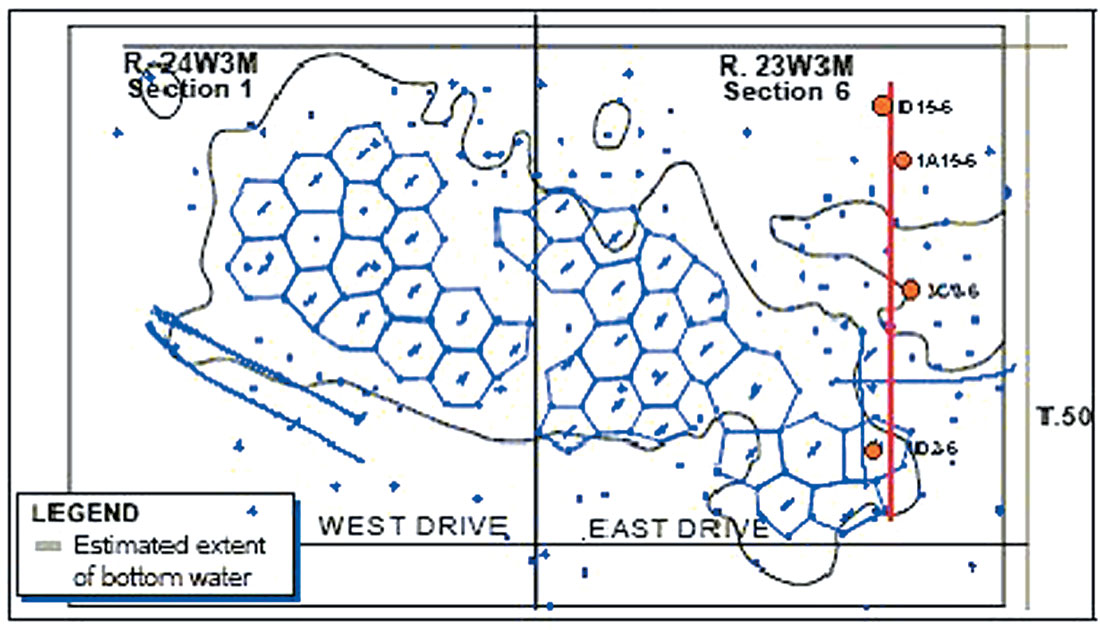
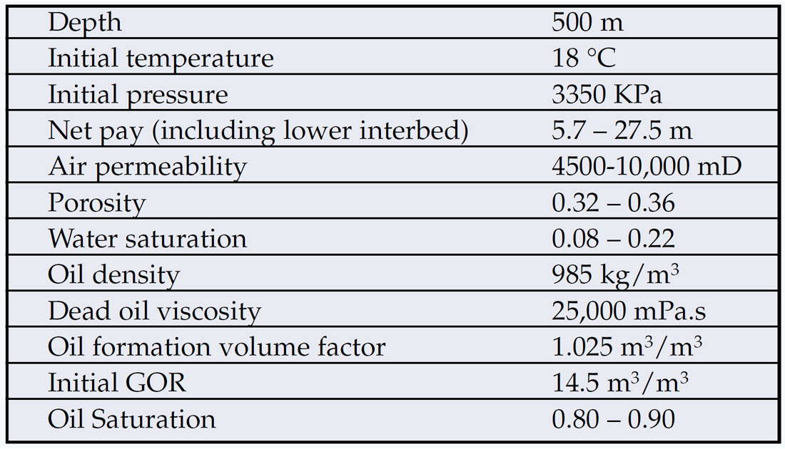
Pikes Peak Field is located 40 km east of the Alberta- Saskatchewan border (Figure 1). The producing reservoir is in the Lower Cretaceous Waseca Formation and is about 500 meters below the surface. The reservoir’s porosity is around 0.32~0.36 with 80% heavy oil saturation. The Waseca production zone has been divided into a homogeneous, well-sorted, predominantly quartz lower unit and a sand-shale interbedded upper unit (Miller and Given, 1989; Sheppard et al., 1998). Figure 2 shows typical logs from well 1A15-6 (X6i in Figure 3). Table 1 contains the basic reservoir properties. Steam drive technology has been applied to enhance recovery by reducing the effective viscosity of the oil. A successful Cyclic Steam Stimulation (CSS) program started at Pikes Peak in 1981. In the eastern part of the reservoir, CSS has been in operation from 1983 until the present. Husky Oil acquired a set of north-south oriented 2D swath lines in 1991. To investigate time-lapse effects, the University of Calgary and Husky acquired a repeat line on the eastern side of the field in 2000.

Reservoir simulation

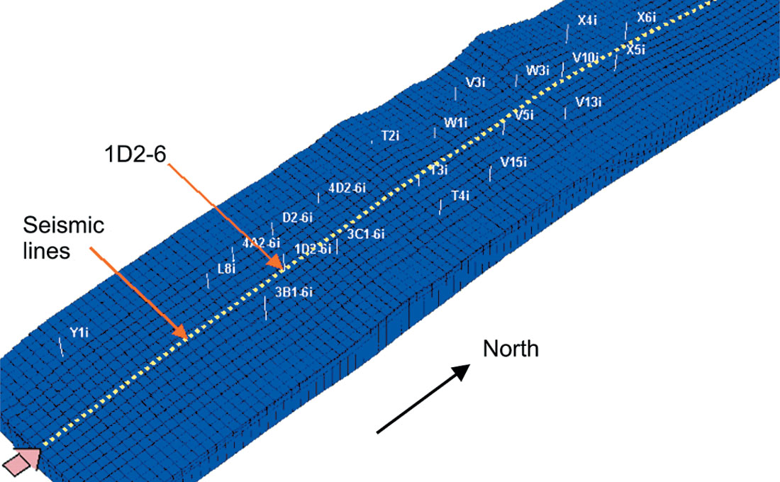
The reservoir model for the present reservoir simulation was built by Husky Oil. The reservoir grid geometry, well locations, and time-lapse seismic line location are shown in Figure 3. The seismic lines are in the middle of the reservoir model in the north-south direction. The grid dimension of the reservoir model is 20 x 20 m horizontally. There are three vertical layers with varying thicknesses. To date we have considered the three layers having individually uniform but distinctive properties that correspond to two upper shale and sand interbedded layers and a lower homogenous sand layer.

CSS started in the southern part of the reservoir in 1983 at well 1D2-6. Average steam injection duration was 10 to 30 days followed by 5 to 10 months of soak and production. The reservoir simulation is based on the injection and production history from January 1981 to August 2003. Temperature increase represents steam progress. The temperature front moves about 5 m to 8 m per year. It spreads faster in the north-south direction than in the east-west direction (Figure 4). Pressure spreads much quicker than temperature (Figure 5). The distributions of pressure, temperature and gas saturation on the 2D profile corresponding to the seismic line location and the resulting synthetic seismic difference section will be discussed later.

Synthetic seismic section

Since the time-lapse seismic surveys were acquired in February 1991 and March 2000, we did seismic modelling only for these two time steps. Using the procedure described in previous seismic modelling work (Zou et al., 2003), we constructed velocity and density models using well logs for regions above the reservoir and calculated the velocity and density within the reservoir using reservoir simulation outputs. Since there is no well that reached the Devonian, we borrowed average log values for the deeper formation from well logs 8 km away from the seismic line. The velocity and density model is shown in Figure 6.

The seismic modelling was performed using point sources and shot gathers for better simulation results. The synthetic data were convolved with a 60 Hz zero-phase Ricker wavelet and NMO stack and post stack migration were applied. The reservoir simulation mesh is different from the seismic grid (CDP interval) so we applied an interpolation to the reservoir simulation output to make the seismic model compatible with the seismic survey. The seismic survey sections and the synthetic seismic sections corresponding to times 1991 and 2000 are shown in Figures 7, 8, 9 and 10. The difference sections between times 2000 and 1991 for the seismic survey and the synthetic seismic section are shown in Figure 11.

Discussion

Figure 11 shows the synthetic difference section (bottom) and seismic survey difference section (top) between time steps 2000 and 1991. The overall match between the seismic survey difference section and the synthetic seismic difference section is very good. Seismic difference banding effects are apparent in both difference sections around the CSS wells. The large difference energy between well V5 and V10 around the Top Cambrian appears on both difference sections. We believe that the broken energy on the seismic survey difference section around the Top Devonian is due to either survey or processing error. The simulated gas saturation, reservoir pressure and temperature distributions are plotted in Figures 12, 13 and 14, respectively, for the three reservoir layers at 1981, 1991 and 2000 time steps. Gas saturation in 1981 was zero. The gas saturation here is for a gas phase constituted of different components such as water vapor and methane. The marked wells are those within 60 m around the seismic line.

According to historical data, wells 1D2-6 and 3B1-6 have been in CSS operation since 1983 and well L8 was in CSS operation from 1983 to 1997. Wells L8 and 1D2-6 were shut in from 1988 to 1992; therefore in 1991 the reservoir in this part was heated up somewhat but was not at a high temperature. Wells 3C1-6, T3, V5 and V10 have been in CSS since 1992, 1995, 1996 and 1997, respectively. Large seismic difference energy appears around the area of these wells because they were not active in 1991. The W wells started CSS in late 1999; not long enough to have an impact on the seismic differences. We can see that there is little temperature change between 1991 and 2000 on the left side of well 1D2-6. We also found gas saturation corresponding to pressure decrease even at low temperatures (CDPs 40 to 80). Difference energy is visible around 600 ms and 750 ms at CDP locations 100 to 200 but is restricted to the top of the reservoir at other CDP locations (CDPs 40 to 80). The red dashed boxes in Figure 11 indicate the areas that have large discrepancy. They may be due to noise in the seismic sections or the limitations of the model. The areas of high gas saturation and high temperature are steam fronts. The wells were very densely located on this profile and therefore there is not much by-passed oil area indicated by this 2D study.

Conclusions

By comparing the saturation, temperature and pressure results from the reservoir simulation with the synthetic difference (Figures 12 to 14), we derived the following conclusions:

1. The areas with gas saturation differences between the two compared time steps show seismic differences because the presence of gas reduces the bulk modulus and bulk density of the saturated rock (Domenico, 1974).
2. Thicker gas zones correspond with larger traveltime delays in the seismic section. The thin gas zones only induce large reflectivity and do not have enough time delay to cause a strong seismic difference in the deeper regions below the reservoir zone (CDPs 40 to 80 on the synthetic seismic difference section).
3. High temperature regions also correlate with areas having seismic energy differences but the correlation is not as strong as the correlation with the gas saturation differences.
4. Pressure spreads very quickly and its value depends on whether the location is in the injection or production stage. The pressure dependence of the seismic data is due to the influence of pressure on gas saturation.

Acknowledgements

We want to thank the CREWES sponsors for their constant support. A special thanks to Husky for contributing their data to us. We really appreciate the input from Larry Mewhort and Don Anderson at Husky and Ian Watson at Imperial Oil. We also want to thank Dennis Coombe and Peter Ho at CMG for their help on reservoir simulation.