Refraction Tomography: A Practical Overview of Emerging Technologies

Near-surface velocity anomalies produce severe distortions in seismic images. If one knew the detailed structure of these anomalies, the best way to tackle this problem would be to perform wave-equation datuming or depth migration from the surface. However, 3-D prestack depth imaging and datuming are computational challenges and highly sensitive to the near-surface model. Therefore, statics application, assuming surface-consistent ray propagation through the near surface, remains the most common approach to account for near-surface anomalies. For estimating the short-period part of statics (so-called residual statics) analyzing the stacking response of reflection data works well. However, estimating the long-period statics, using reflection data alone, is more problematic. Therefore, solving for the near-surface velocity model from refraction data, followed by calculating predominantly long-period statics, is customary in seismic processing.

Refraction statics have long been implemented using delay-time methods. For example, the generalized reciprocal method has been widely applied to 2-D data. Unfortunately, for 3-D seismic, it is difficult to apply due to the lack of reciprocal data. However, the concept of delay times is useful for 3-D refraction statics calculations by assuming first arrivals to be the onset of head waves propagating along the refracting interfaces of locally flat layers on the scale of the offset range (Figure 1). First-arrival picks are decomposed in a surface-consistent manner into delay times and refracting-layer velocities. These are then converted to layer thicknesses assuming a critical angle of incidence at the refracting layers. The model used in the delay-time method is also used in head-wave tomography, as implemented, for example, in Generalized Linear Inversion (Hampson and Russell, 1984). In this approach, instead of the two-step inversion via delay times, traveltimes are inverted directly for layer thicknesses and velocities after ray tracing of head waves.

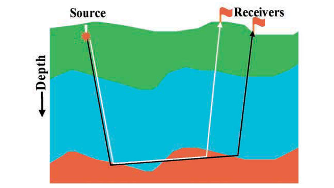
Head-wave methods are in general robust because the relationship between the delay times and the observed traveltimes is linear. However, in areas with complex geology and rough terrain the layered model typically employed is often too simple to explain important data features. Furthermore, since head-wave methods do not account for nonlinear moveout of first arrivals, it is often necessary to limit the offset range. This limiting of the offset range contributes to a fundamental velocity/depth ambiguity. To address this issue, it is common practice to specify the weathering velocity prior to depth estimation (Hampson and Russell, 1984).

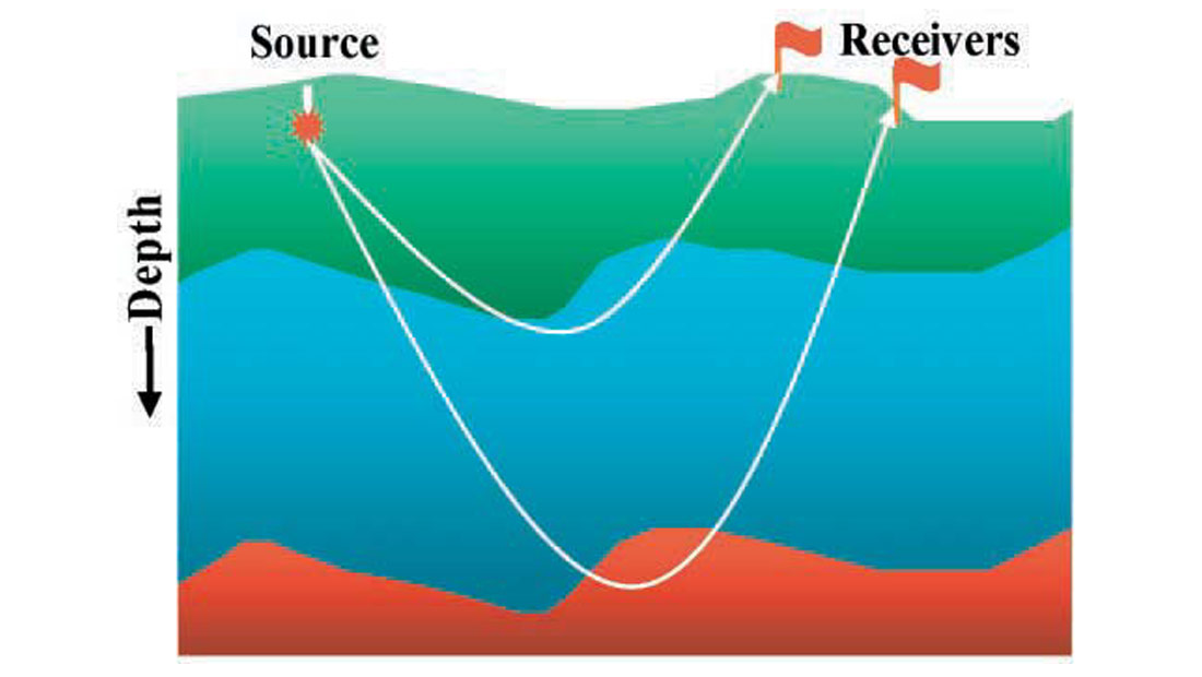
Recently, diving-wave, or turning-ray, tomography has become a popular alternative to head-wave methods (Zhu et al., 1992; Bell et al., 1994; Osypov, 1998; Zhu et al., 2000). In this approach, the medium is typically parameterized as a number of cells. Turning rays are then traced through the model, and traveltime residuals are inverted for velocity perturbations in every cell crossed by rays. Since this method adds more degrees of freedom to the model, it generally fits the observed first-arrival moveouts better than headwave methods. Specifically, the model for diving waves includes vertical velocity gradients (Figure 2). This accounts for the nonlinear moveout of first arrivals and allows for the solution to incorporate a wider offset range. However, the relationship between the model parameters and the traveltimes becomes nonlinear due to the significant sensitivity of turning-ray paths to the velocity model. The nonlinearity is usually handled by iterating the ray tracing and the model updating using a local linearization. This makes the tomographic results sensitive to the initial model. Since the quality of the initial model depends on the analyst’s expertise, this may cause a bias in the final solution. The above issues are exacerbated when the data quality is poor. In other words, the results of diving-wave tomography are usually more sensitive to pick errors than are the solutions of head-wave methods.

A desirable goal for diving-wave tomography is to reformulate it as a linear problem in order to remove the initial-model dependency. Toward this goal, traveltime inversion in the τ-p domain is very attractive, as it possesses an inherently linear formulation. Different forms of τ-p traveltime inversion have long been used in earthquake seismology. However, the practical application to 3-D refraction tomography, until recently, was constrained by a 1-D assumption. Figure 3 illustrates a 1-D inversion producing a unique velocity/depth model from the observed traveltime curve under the assumption of velocity increasing with depth. For the velocity model shown in Figure 3d, the traveltime vs. offset curve is plotted in Figure 3a. Given the observed traveltimes along this curve, there exist two particular approaches for solving the inverse problem to estimate the implied velocity model. One option is to take a derivative of the traveltime curve to calculate apparent slowness as a function of offset x (Figure 3c). The apparent slowness in the 1-D case corresponds to the ray parameter, p. In the x-p domain, one can then apply the Herglotz-Wiechert (H-W) formula (Aki and Richards, 1980) to derive the depths of penetration for diving waves corresponding to the ray parameters for the different offsets. Since the p value corresponds to the physical velocity at the turning point, this transformation provides an estimate of the desired velocity/depth function in Figure 3d.

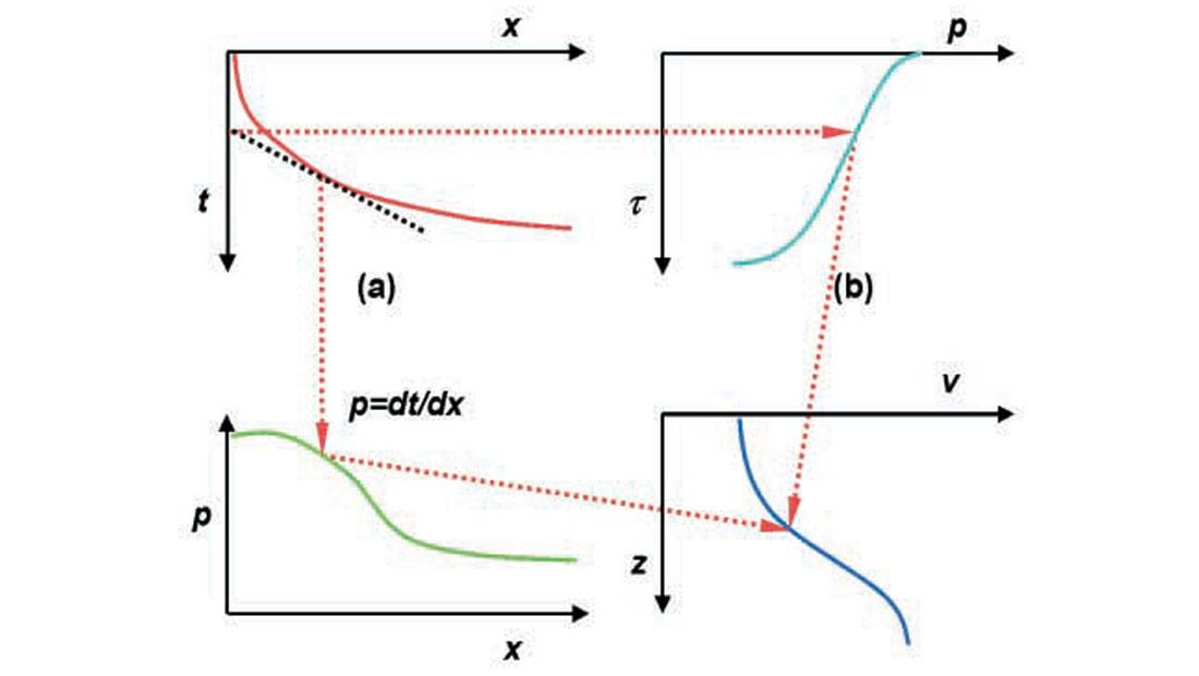
The other solution of interest for the inverse problem, is to calculate intercept times, τ, for each p (Figure 3b). Then, one can apply another form of the H-W formula in the τ-p domain to estimate the velocity/depth model in Figure 3d. A discrete form of this H-W transformation corresponds to the ray geometry for head waves, yielding a multi-layer delay-time relationship. Numerically, the HW transformation in the x-p domain is more accurate and stable for continuous velocity functions. However, the transformation in the τ-p domain is better for treating velocity discontinuities. This leads us to adopt a hybrid form of the H-W transformation to invert both head and diving waves for a velocity model with both sharp velocity transitions and mild vertical velocity gradients. This transformation may be extended to the case of velocity inversions, but the solution becomes non-unique.

In order to extend this hybrid approach to 2-D and 3-D, one has to decompose the observed first-arrival traveltimes into an equivalent τ-p representation. I introduced a form of refraction tomography without ray tracing using a local, 1-D H-W transformation applied to the traveltime curves obtained by the decomposition of first arrivals (Osypov, 1999). Later, I modified the decomposition by exploiting the tomographic-like integrals coupled with a 3-D extension of the hybrid H-W approach (Osypov, 2000). This founded the basis for a new τ-p refraction tomography method.

I implement τ-p refraction tomography as a two-step process. First, I decompose the first-arrival picks to a best-fit τ-p representation in 3-D using a linear inversion that does not require any explicit ray tracing, cell parameterization, or initial model. The second step is a separate, local inversion that involves the estimation of the 3-D velocity/depth model from the derived τ-p representation. This model building process may incorporate a priori information such as upholes.

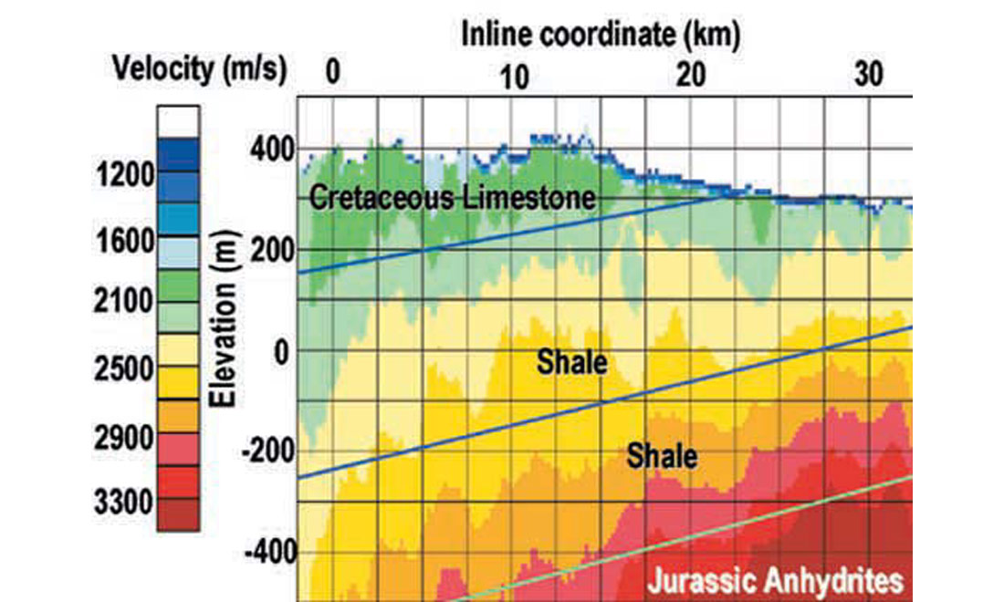
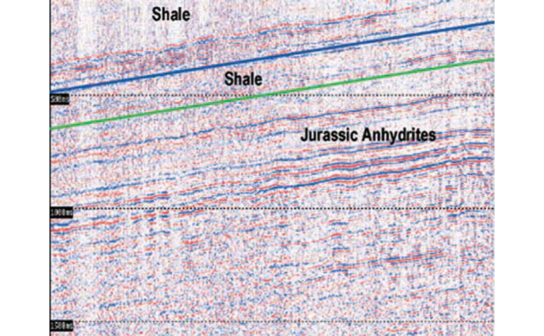
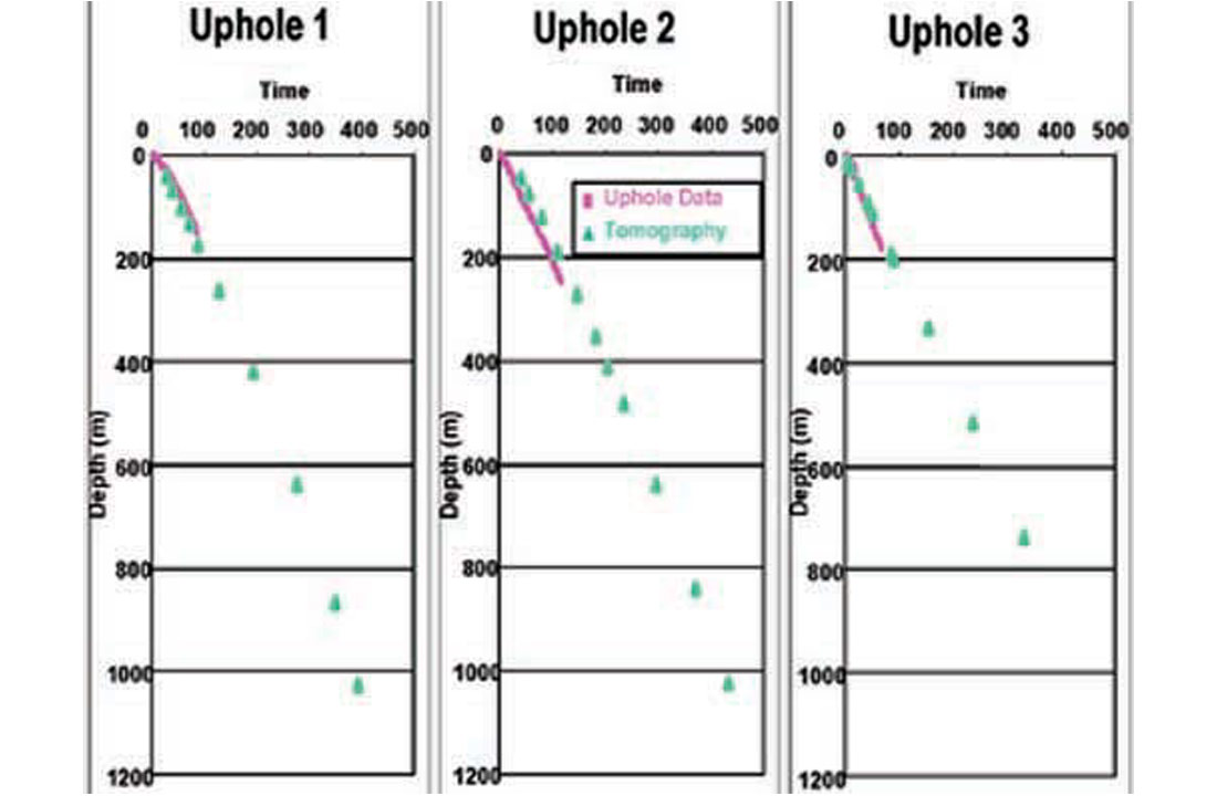
Figures 4, 5, and 6 show the results of applying τ-p refraction tomography to a data example from Tunisia (courtesy of Petro-Canada). The results demonstrate a good agreement with the independent geologic and uphole information. Other examples comparing the accuracy and robustness of different forms of refraction tomography may be seen in Osypov (1998, 1999, and 2000).

In conclusion, τ-p refraction tomography is an emerging technology that complements other well-known methods for modeling the near surface and producing static corrections. This method of traveltime inversion differs from conventional tomographic approaches in that it performs no explicit ray tracing, although its formulation is implicitly based on ray theory. The approach combines the robustness of delay-time methods, as it does not require an initial model, and the flexibility of tomography, as it inverts both head and diving waves over the complete offset range.