Quantitative estimates of fracture density variations: further perspectives

Summary

We have undertaken a quantitative investigation of the accuracy of surface seismic attributes in predicting fracture density variations within the Nordegg Formation in West Central Alberta. These results were first discussed at the GeoCanada 2010 convention (Hunt et al, 2010) and also published in The Leading Edge (Hunt et al, 2010). We showed that the Nordegg was fractured, that those fractures were likely important to production, and that we seemed to be predicting those fractures in a statistical manner with Azimuthal AVO (AVAz) and curvature attributes. Further discussion about the sensitivity of the AVAz attributes to sampling also took place at the 2010 SEG Convention (Downton et al, 2010).

These studies were quantitative in nature, relying on microimage log (image log, or MI) data taken from two horizontal wellbores as well as microseismic data. It was felt that these data formed a large enough population to draw some objective conclusions about the attributes. It behooves us to further use this control to attempt to gain a deeper understanding of the fracture-predicting attributes, their strengths, their weaknesses, and potential best practices around their use. We take a critical look at our work in an attempt to provide this perspective. This effort shows that a rock property rescaling of the curvature attributes might improve their relationship to relative changes in fracture density, and that sampling and the handling of issues related to sampling are critical in achieving more accurate AVAz estimates.

The difficulty in drawing conclusions

Drawing conclusions is a perilous undertaking. As human beings, we cannot escape our biases completely. We desire results that help us in some way. Objective, quantitative testing following the scientific method provides a structure that can minimize that bias. Fracture predictions are particularly perilous for a number of reasons:

1. We have a limited amount of control data.
2. The control data we do have is limited in accuracy, applicability, and typically has different support from our surface seismic data.
3. We have a very limited history of quantifying fracture predictions, and most of that history has involved a posterior analysis.
4. We really want to be able to predict the fractures (which means we are biased towards saying we can).
5. We have little clue as to what the answers should look like.

These challenges make an objective, quantitative approach to fracture analysis much more important. We touch on some of these problems within our own study, and talk a little about statistical certainty and geostatistical issues relevant to the work. We also show just how difficult it is for anyone to evaluate or quality control the accuracy of azimuthal attributes in the absence of control data.

Weaknesses of the attributes and what we can do about it

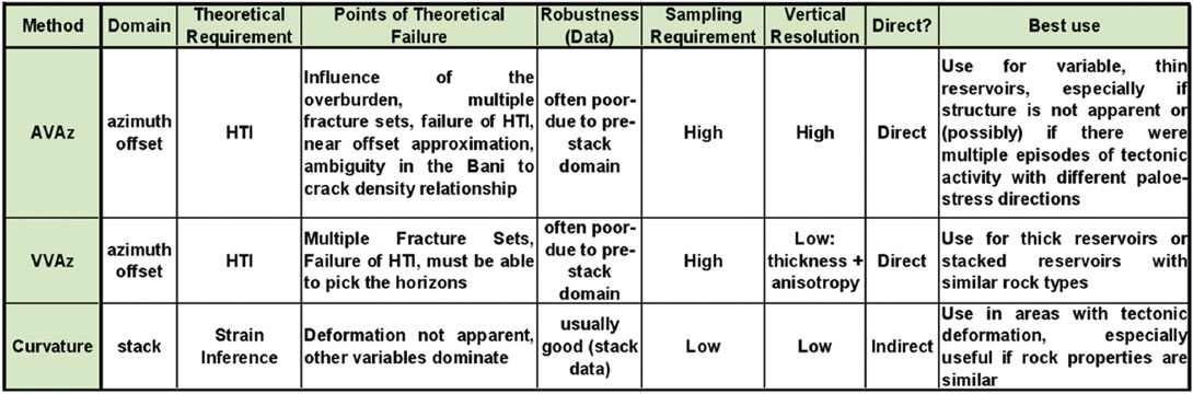
None of our attributes are perfect. Curvature is performed on robust data but is a fracture inference based on one of many causal variables. AVAz is a direct indicator of fractures but has narrow limits of applicability (i.e., unforgiving theoretical requirements) and is performed on less robust, poorly sampled data. Velocity variation with azimuth (VVAz) has some of the same problems as AVAz but has lower resolution. We delve into these issues further and consider two strategies:

1. We accept the weaknesses of the attributes, but by carefully considering their strengths and weaknesses, we either choose the best one for the task, or choose the best combination. We give some example ideas of this in the talk. Table 1 below illustrates a summary of the relative strengths and weaknesses of the attributes.
   
   Curvature and azimuthal methods have converse robustness versus directness characteristics, which make them worthy of complementary use under a variety of data quality and structural settings (Hunt et al, 2010). This can take the form of multivariable solutions or cross plotting. Even the azimuthal attributes have differences in usage: VVAz may not suffer some of the same theoretical weaknesses as AVAz, but has lower resolution. Strategies around the use of these two azimuthal attributes depend on the situation: if the reservoir is thick with similar rock properties (such as a thick set of stacked sands), VVAz may have an advantage. If the rock properties vary vertically and vertical resolution is important, AVAz may offer advantages. VVAz requires the picking of events from which the velocity variations are measured, so the spacing and robustness of those picks can become very important practically.
2. We attempt to minimize the weaknesses of the attributes by improving them. These improvements are reached through either modifying the attributes themselves, or modifying how we extract them.
   1. Curvature depends on the strain inference. How could we use our knowledge of the causes of fractures to strengthen the causal relationship and create a new variation on curvature?
   2. The effects of sampling on AVAz are profound. AVAz anisotropy measurements are difficult to evaluate in the absence of control data, which makes their quality control problematic. We will quantitatively evaluate our methods of borrowing data and scaling azimuth and offset bins through the use of correlation to image log data as in Hunt et al (2010). We compare some of these:
      1. Superbinning 1x1, 5x3 binning
      2. Special scaling and binning (Canning and Gardner, 1998) (i.e., intense, expert intervention)
      3. Interpolation with and without superbinning iii) Interpolation with higher effort
   3. c) How do COV methods of AVAz estimation compare to AVAz from azimuthal sectored migrations?

A new curvature attribute: L/M (or) Brittleness rescaled curvature

Curvature is a useful attribute set for making predictions regarding fracture density (Hunt et al 2010). Curvature data can infer variation in fracture density based on three asumptions: the rock is brittle and fails largely due to fracturing, an increase in curvature implies an increase in strain, and an increase in strain implies an increase in fracture density (Nelson, 2001). Nelson (2001) describes that there are many other causes of fracture density variations, which Hunt et al (2009) summarized in a table, reproduced below as Table 2.

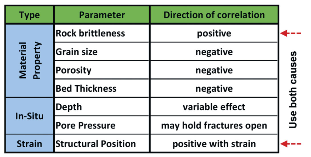
These causal variables are many, and have been verified in the lab and in outcrop (Nelson, 2001). The applicability of curvature to infer fracture density variations depends heavily on how much these other causes vary within a study area. This limitation can be visually assessed by inspection of the curvature attributes. Figure 1 shows the low-resolution most positive curvature attribute along horizontal wellbore A from our fracture density study (Hunt et al, 2010). The Viking is depicted by the uppermost red horizon, and demarks the start of the Early Cretaceous section, which has higher rigidity than the overlying shale section. The Nordegg is depicted by the lowermost red horizon, and denotes the boundary between the Early Cretaceous and the higher rigidity Jurrasic section.

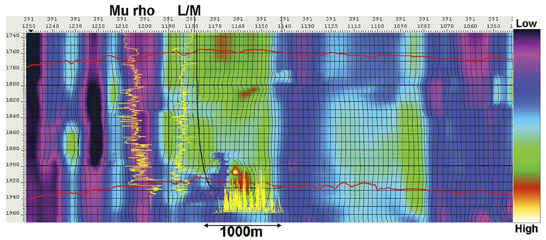
This curvature attribute was computed volumetrically with methods described by Chopra and Marfurt (2007). The attribute has a strong vertical striping, which is simply the measurement of curvature over the anticline that well A was drilled along. As a fracture predictor, some vertical similarity is expected. However, we also know from the lambda rho divided by mu rho (L/M ratio) attribute logs shown that the rock properties vary significantly above and below the zone of interest. The vertical similarity may therefore make sense from a curvature point of view, but it ignores the effects of the varying material properties on fracturing as we move up and down stratigraphically. Goodway et al (2006) showed that the rock’s brittleness can be reasonably described by the L/M ratio or by the closure stress ratio:

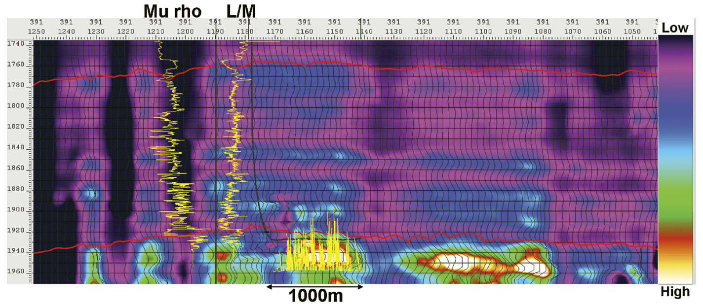
where σ_x is horizontal stress, σ_z is vertical stress which yields similar behavior to L/M ratio. Both L/M ratio and closure stress relate how difficult it will be to fracture a rock. These indicators depend heavily on mu. Difficulty to fracture, and likelihood of fracturing obviously go together, so these ratios should be causally related to fracture density variations. These parameters can be estimated from seismic data (Goodway et al 1997). Figure 2, is the mu rho attribute from the same seismic as in Figure 1, and Figure 3 illustrates the L/M ratio.

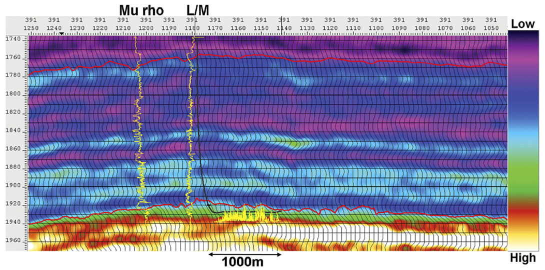
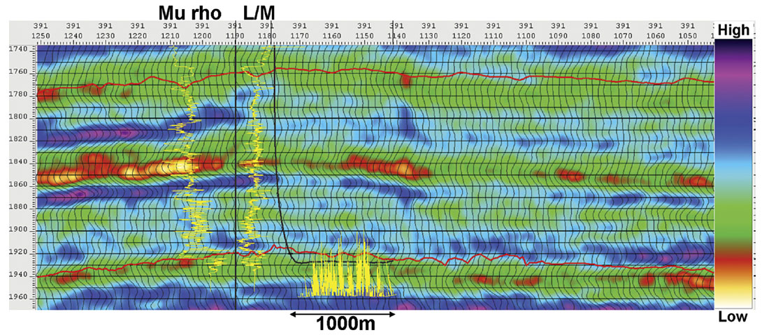
The mu rho attribute shows an obvious step change at the Viking level (the upper horizon) and at the Nordegg level (the lower horizon). The low-rigidity Poker Chip shale overlies the Nordegg, and exhibits a strong contrast to the rigid, chert dominated Nordegg. These variations are remarkable, and suggest rock property variations will likely be an important causal variable in the distribution of fractures.

The L/M ratio attribute has a more complex appearance, but illustrates the greater frac-ability of the Nordegg by the lower values of L/M ratio in the zone. Based on the L/M ratio and mu rho data, we expect that the Viking should fracture more readily than the overlying shales, and the Nordegg should fracture more readily than much of the overlying Cretaceous section.

To strengthen the vertical or stratigraphic discrimination of the inference from curvature, we want to combine these rock property attributes with the curvature attribute. Referring back to Table 2, this combined attribute will consider two causal variables of fractures: strain and brittleness, rather than just strain. The combination could be perfomed in a variety of ways, however Goodway et al’s (2006) reformulation of the closure stress equation in terms of Lame parameters suggests the form of the equation we chose to use. The closure stress equation is re-written below in simplified terms:

Closure stress = closure stress ratio[effective stress + 2μ (tectonic strain term)] +pore pressure term

If we remove the effective stress and pores pressure terms, we create a curvature rescaling expression with the following similar form:

Rescaled curvature = brittleness term [Curvature]

Figure 4 shows a rescaling of the curvature attibute with the mu rho estimate as the brittleness term. This scaling method does not require us to solve for any weighting coefficients, and is a simple starting point for dealing with the problem.

This new attribute still exhibits some vertical striping, but also has characteristics of the rigidity estimate. A better combination would be made from the use of either the closure stress ratio or L/M ratio. Figure 5 shows a rescaling of the curvature attribute with the L/M ratio estimate as the brittleness term.

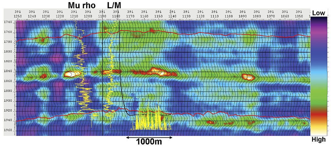
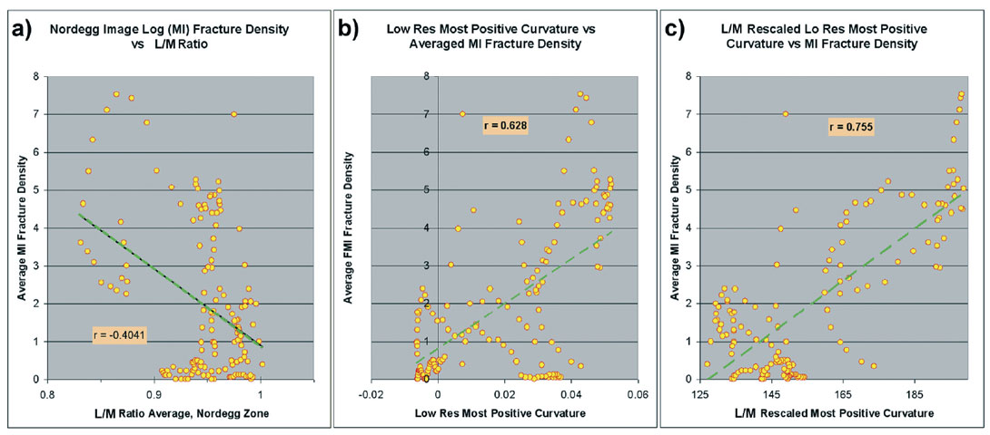
We will refer to this new attribute as L/M rescaled curvature. As with the mu rho rescaling, it retains some of the characteristics of curvature and some of the character of the L/M ratio. The rescaling is non-linear and uses an arbitrary damping that affects the relative contribution of each attribute. The new attribute should contribute to the ability to make relative fracture density inferences in different rocks with the same curvature. Rocks of different brittleness that have the same curvature value may now be more correctly inferred as having different fracture densities. This might be more obviously viewed vertically in a thick folded section. We expect this result to be less obvious viewed horizontally within the same general rock type, such as in our Nordegg horizontal wells. Nevertheless, we compared the image log fracture densities of wells A and B to the attributes extracted along the wellbore as described in Hunt et al (2010). Figure 6 illustrates the scatter plot from that extraction. The L/M ratio of Figure 6 a) has a somewhat weak negative correlation to fracture density, but the trend of the correlation makes physical sense. Lower values of L/M ratio tend to correspond to the highest fracture density. The low-resolution most positive curvature attribute of Figure 6 b) correlates positively to the fracture density. The L/M scaled curvature attribute shown in Figure 6 c) has a superior correlation to either of the others. These correlations provide some empirical justification for combining the curvature and L/M variables in some fashion, and the trends of the correlations match our broad theoretical expections.

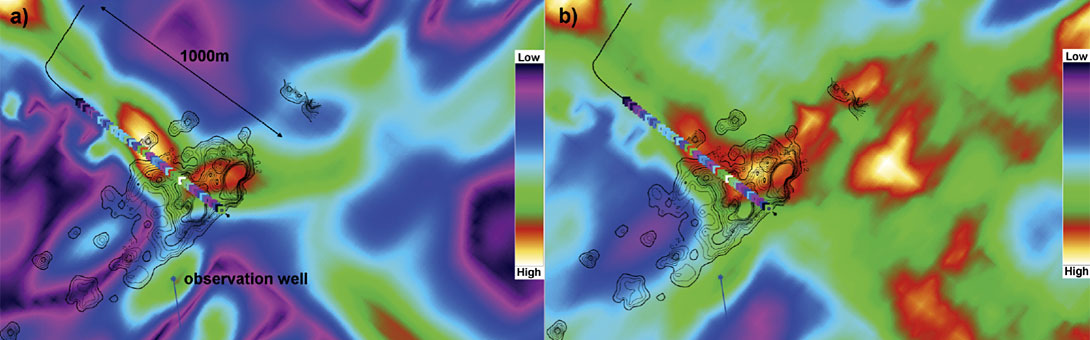
Hunt et al’s (2010) work also attempted to use microseismic data as a validator of fracture predictors. We extracted map comparisons of curvature and L/M rescaled curvature in the area of the microseismic. A comparison of those attributes to the microseismic cumulative event moment contours is shown in Figure 7.

The L/M rescaled curvature attribute has a much higher correlation to the microseismic data. Further testing should be done with this new rescaling scheme. Closure stress ratio rescaling should produce similar results, although this should be tested. Image log data from vertical or deviated wells should be correlated to both curvature and brittleness rescaled curvature attributes to determine whether the improvement is more obvious in vertical section (which we predict). This scaling method is only a simple first step: more work on the analytic formulation for this attribute would be a desireable future development. A more complete approach could also consider the effects of pore pressure and depth in the combined brittleness and strain expression. The goal here is to consider as many of the causal factors of fracture density variations into an indirect fracture prediction expression that is formulated according to rock mechanical theory.

AVAz sensitivity to sampling

Azimuthal attributes such as AVAz are sensitive to sampling (Downton et al, 2010). Hunt et al (2008) illustrated that interpolation prior to imaging improved the accuracy of AVO estimates on this same coarsely shot 3D survey. The source lines have an average spacing of 660m, and the receiver lines have an average spacing of 600m. AVAz should be even more sensitive to irregular, sparse sampling and imaging noise due to the requirement of populating the azimuth dimension in addition to just the offset dimension. AVAz studies demand careful consideration of these sampling needs. Almost any land 3D survey requires bin borrowing in order to populate the required offset and azimuth data. Interpolation can be used to minimize these problems although even with interpolation, bin-borrowing, area weighting and scaling may still be required. Alternatively, Common Offset Vector (COV) methods (Cary, 1999) may be used. This requires regularly sampled source and receiver line spacing and relatively small tile sizes (to avoid introducing an AVAz footprint (Downton, 2010)). Here again, interpolation can be used to fully regularize and reduce the offset vector tile size of COV surveys to help alleviate the above issues. We tested this hypothesis by processing the data with different interpolation/migration flows and compared the resulting AVAz estimates with the image log data from the well control. The AVAz anisotropic gradient (Bani) results are compared in Figure 8 along well A from Hunt et al’s (2010) study along with the image log fracture density data.

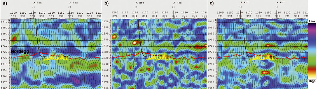
We compare a result with 5 by 3 bin super-binning, area weighting and migration in Figure 8 a) scaling to a similarly super-binned result that had special effort in the binborrowing in Figure 8 b). This special effort included manual inspection and intervention with regard to the azimuthal bin population. We also show the results obtained if we interpolate the data and employ bin-borrowing. It is clear that the high-effort result of Figure 8 b) is superior to the result of Figure 8 a). The interpolated result in Figure 8 c) is the best. We evaluated the quality of the results objectively through correlation to the image log fracture density data as described earlier. Those results are shown in Figure 9.

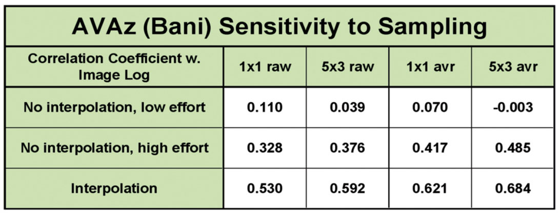
It is clear that the scatter plot resulting from the interpolation version in Figure 9 c) is the best, while the lower effort 5 by 3 superbinning result fails to show a statistically meaningful scatter plot. The correlation coefficients from this analysis are shown in Table 3, and support this observation.

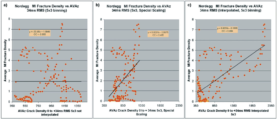
The correlations were carried out against averaged and raw image log data in consideration of scale differences in the data, and we also looked at data without superbinning. In this experiment, interpolation was crucial, but superbinning of the interpolated data also seemed to be of use. The sensitivity of the results to level of effort in binning and scaling is remarkable and scary.

Best (better?) practices

In considering the strengths and weaknesses of the attributes and thereby modifying our processing of them, we are clearly suggesting best practices. Given the early nature of the work, we should emphasize that all we can really do is point to what we hope are better practices. We will talk about interpretive practices as well. In particular, we will address the sensitivity these attributes have to the way we pick them on the workstation, and what that may tell us about them.

In order to validate the predictions of fracture density, we have compared image log data to surface seismic data attributes. This comparison is made difficult by the differences in scale of these data types. The image log data is sampled at a decimeter scale while the seismic data bins are 30m by 60m in size. Moreover, the seismic attributes are commonly calculated on data that is either spatially filtered or binned in some further manner that enlarges the true sample size even further. Dealing with these problems involves up-scaling of the image log data. Changes in scale or support are well known geostatistical processes, and were of some issue in this work. Figure 10 illustrates the image log data from well A and a few different averaging schemes used to change the support of the image log data to the same scale as the seismic data. The final, averaged image log data used a smoother that was several seismic bins in length. This was done in appreciation of the processing effects mentioned earlier.

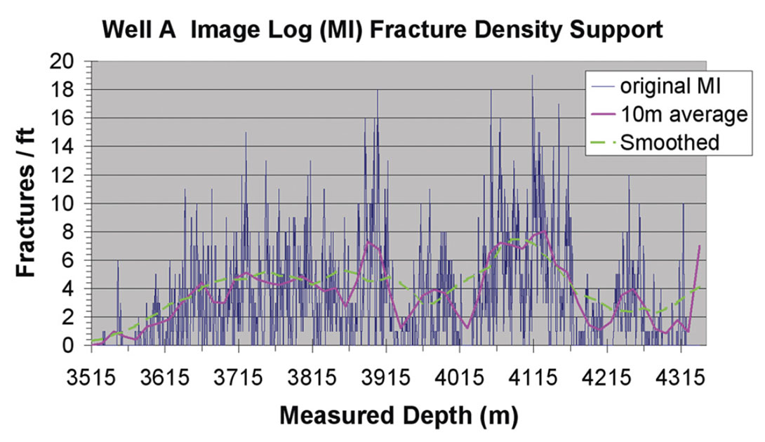
Changes in support typically involve averaging of the data. We experimented with several different linear and non-linear averaging schemes, and found that they all had a similar effect on the data correlations provided they achieved a scale such that they respected the filtered bin size of the attribute data. This is not to say that the exact method of support change is unimportant: it can be. Changes in support reduce the variance of the data, and can affect the skew of the data distribution. The image log data has a highly skewed, power law type distribution. The simple methods of up-scaling that we used did act to reduce the skew of the image log data distribution somewhat. We recommend that more sophisticated methods of change in support be utilized in the future. Methods that retain the shape of the image log data distribution would likely be better. Some of these methods are described by Isaaks and Srivastava (1989). We might also consider handling the support differently for different attributes in recognition of the amount of spatial filtering that each attribute might have.

Conclusions and what we hope

Fracture prediction can be performed using curvature and azimuthal attributes in a statistical sense. The accuracy of the results depend on what the data quality and sampling allows as well as the degree to which the manner of fracturing in the rock meets theoretic requirements. Consideration of the strengths and weaknesses of the attributes allows for the most advantageous attribute to be chosen, or encourages advantageous combinations of the attributes. We also demonstrated that the curvature attribute may infer fracture density variations better if rescaled with brittleness estimates from the data. This should be tested further, and with more analytic approaches to the rescaling.

We also showed that AVAz is very sensitive to sampling, binning, and interpolation. On this data, both interpolation and super-binning were required. Is this a promotion of interpolation or an indictment of our sampling? Although the results certainly support the importance of interpolation combined with careful handling of binning and scaling, they also are suggestive that our poor and irregular sampling has put us at risk. Interpolation should not be so important: if our results on this survey are this bad without it, we have really put ourselves into a desperate position. While we recommend applying interpolation for all AVO and AVAz processing flows, we caution against over-reliance on it. It is possible that we will encounter situations which cannot be fixed by interpolation. We do not create data with interpolation, we only fill in the holes with a reasonable estimate. If our data borrowing or estimation distances get too large (and we may not know how large is too large), we risk misapplication and error. This survey has coarse line spacing. These effects would likely be reduced if the survey was shot with finer source and receiver line spacing. While we stand behind our recommendation to always use interpolation for land 3D surveys if AVO or azimuthal analysis is to be considered, we also recommend that tighter source and receiver line spacing be used in any new shooting wherever these methods of analysis might be employed.

There are a number of other practices that we could improve as we move ahead in our understanding of fractures. The windowing of the attribute data can be important, and needs to be considered relative to the way in which the attribute is calculated. The effect of changes in support between data types should be handled carefully, and likely with methods that respect the original data distributions. Commercial software developments that consider these notions will be helpful in enabling more efficient tests of these concepts in the future. This development may increase the likelihood of further and more frequent quantitative tests.

We hope that this discussion adds to the general understanding of fracture prediction. We also hope that some of the questions we discuss encourage further work from other people who have their own control data. While this study has statistical value, it is one study, and with one set of control. Other studies that extend or modify these methods, or use entirely new and better approaches, would be most desirable.